jason's hyperion blog

essbase from the trenches

A REST API Primer for EPM Users & Developers

There’s a lot of excitement in the EPM world these days when it comes to REST APIs – and rightfully so. As a developer heavily invested in the EPM space I am excited about some of the possibilities these new APIs offer – and what they will offer in the future. But all of this great new REST API stuff can be quite daunting – how does it work, why should you care, where does it fit in with your overall architecture, and so on. And with ODTUG‘s Kscope18 just around the corner I thought it might be useful to write a primer – or a crash course of sorts – for the EPM professional on what all this REST API business is about. Also be sure to check out one of my presentations at Kscope this year as I will be discussing the OAC Essbase REST API, how to use it, what it does, and more.

REST APIs in a Nutshell

Many services in the Oracle EPM cloud space now have a REST API. PBCS was one of the first Oracle cloud services to get the ball rolling in this regard. Others have followed, such as FCCS, OAC, and more. But when someone says they have a REST API, what exactly does that mean?

For starters, it means that for the given service, there exists a way to programmatically interact with it. This is essentially the API (Application Programming Interface) aspect: as the consumer of the API, you might not and in fact often don’t care how it works, just that you have the capability to ask some black box to perform some action. For instance, maybe you want to run a calc script or a business rule in PBCS. As the consumer/user of the system, you don’t care how this happens or any of the gory details, you just want to know that you can tell it to do something and it’ll do it. It’s a black box to us because we don’t have any sense of the gory details: where things are on disk, how the script is written, which dimensions are dense and sparse, or anything.

The REST piece of things is a bit more nuanced. This means that the mechanism used to communicate with the service is HTTP. Yup, this is the exact same mechanism that your web browser uses to communicate with all of the websites that you browse. As it turns out, not only is HTTP a great protocol for humans to use to talk to computers around the world (a la the World Wide Web), it turns out that it’s amazingly effective at letting computers talk directly to other computers.

By way of contrast, for those of you that have been in the Essbase world for awhile, you might be aware of vaguely aware of this notion of a Java API that Essbase has that let’s you do just about anything you want with Essbase. Indeed, the Essbase Java API is quite capable and powerful, particularly if you already know Java. But what if you don’t know Java or your company has expertise in another programming language, such as C# or Python or something else? This is one of the key awesome things about REST APIs: they’re programming language agnostic.

So, whereas in the past you may have been dependent or beholden on some company to provide a Java JAR, or a DLL, or whatever, providing a REST API is effectively them saying, “Hey, use whatever language you want – you’re not dependent on us.” And you might not want to use Java either, which is also fine – most modern programming languages have very robust support for working with both HTTP and REST, be it Java, C/C++, C#, Python, JavaScript, Groovy, PHP, Swift, or something yet to come along.

What’s this JSON stuff?

JSON is generally used as the format of requests and responses to and from the REST service. JSON originally got popular by way of the JavaScript programming language (hence the name, JavaScript Object Notation). JSON lets you model both simple and complex data: arrays, lists, and objects, numbers, strings, and more. If you are familiar with XML, think of JSON as a less-verbose and lightweight way of defining data. In fact, anything that you can represent in XML you can represent with JSON. Here’s an example of the same data structured as both JSON and XML.

As another simple example, let’s say that we want to make a request to a service and that we’ll use JSON to specify the application, database/cube, and a data file to load:


{
  "application":"Sample",
  "cube":"Basic",
  "dataFile":"calcdat.txt"
}

In JSON terms, this is a pretty simple data structure. It’s an object with three keys: application, cube, and dataFile. The equivalent data structure in Java would be a Map<String, String>. Actually, because JSON supports objects of arbitrary complexity, the equivalent Java data structure would be Map<String, Object> (since the values can be strings or numbers or other objects).

I want to make a quick-aside on one of the reasons that JSON is a great format for exchanging data, particularly in APIs: it offers the developers and consumers of the web service a lot of flexibility when it comes to evolving and enhancing the API. With more traditional APIs, making changes would often result in backwards incompatibility and it would break things. It would often necessitate having to create and distribute a new library/module for your end users. But when using the JSON format, you can generally add in new keys/objects and older clients will still generally just work as they always did. For example, let’s say that the previous JSON example was the data format to specify loading a local data file on a cube, but now the developers (Oracle) want to enhance it with a new option that will automatically calculate the cube after loading the data file:


{
  "application":"Sample",
  "cube":"Basic",
  "dataFile":"calcdat.txt",
  "calcAfterLoad: "true"
}

You can see that there’s a new key called calcAfterLoad that takes a boolean (true/false) value. Again, old clients will continue to work without changes (the server will assume that the calcAfterLoad setting is false if unspecified), and clients that wish to upgrade can take advantage of the new functionality when they’re ready for it.

Because of the flexibility of the JSON data exchange format, you tend to see REST API versions evolve much more quickly than traditional APIs (as new things are added), while also [nicely enough] not actually breaking backwards compatibility. When fundamental changes need to be made, it’s pretty typical for the company/service offering the REST API to just create a new REST API side-by-side with the existing one (perhaps denoted with v1, v2, v3, etc.), and then tell developers that the old API is “deprecated”. To say something is deprecated is basically programmer-speak for “you can still use this for now but we reserve the right to get rid of it in the future, also, please don’t write any new code that uses these deprecated methods, for the aforementioned reasons”.

Okay, how about this cURL thing?

It’s quite common for services with a REST API to provide documentation on how to use the API in various forms. They’ll often include examples of request and response to various API methods, and they’ll also quite often show examples using a tool called cURL. cURL is a command-line client that makes HTTP requests to a given URL, almost exactly the same way that your web browser communicates with websites. cURL is shipped by default with Linux and macOS and is available as a download for Windows machines. It’s popular for many reasons. For starters, it’s free. It’s universally available, very capable, and very easy for developers/testers to copy/paste/edit examples and get started with an API.

Where does epmautomate fit in?

The EPM Automate tool is a command-line tool that can be used as part of automation. It ran load data, run business rules and more. It might not always be pretty but it gets the job done. The relationship of EPM Automate to the REST APIs is pretty direct: it uses them. So effectively, EPM Automate is a consumer of the REST APIs itself. This is also an example of what is called “dogfooding” in the software world: force yourself (the makers of EPM Automate) or one of your teams to use the functionality provided by another team (the PBCS or whichever service’s REST API). This is a good thing in the software world because it kind of forces you to actually test out the stuff you’re making in a real world way, instead of just pitching it over the fence to your end users and saying ¯\_(ツ)_/¯ in case something doesn’t work as expected.

So I can use EPM Automate and we’re all good, right?

Kind of. For many people, automation with EPM automation or even putting in calls to cURL in their automation will get the job done. And this will be good enough in many instances. I would add some caution to this approach, however. One, error control is notoriously complicated when using these low-level mechanisms. Things are fine when everything executes as it should, but when a single statement in a multi-line script fails, what happens? Intrepid developers will put in some guards to check the output or result code and alert the user as to an issue, and this will mitigate the risk of using these tools for many people – but not all. Wherever possible, I advocate for using a higher-level language (Java, Python, Groovy, whatever) for consuming the REST API, and then benefitting from the very advanced error handling and control flow that those languages give you. This is why I wrote the PBJ library – a high quality 100% Java, open-source and freely available Java library for working with the PBCS REST API.

The idea behind this library, and of designing a similar library in your chosen language is that it takes care of the details for you, and everyone benefits from getting to use such a library. For example, you’ll notice nothing to do with JSON, HTTP, REST, or anything in this simple example that calls a business rule:


PbcsClient client = new PbcsClientImpl(server, identityDomain, username, password);
PbcsApplication app = client.getApplication("Vision");
app.launchBusinessRule("AggAll");

Something that’s really great about having a solid, high-quality Java library as your foundation library is that you can use it transparently with other JVM languages, including Groovy, which is increasingly popular in the EPM world as an all purpose utility language. You can check out an example of using the PBJ library with a super simple Groovy script.

Wrapping Up

It’s an exciting time in the Oracle world with all of this new stuff with the cloud, REST APIs, and more. But it can also be quite daunting to keep up and more importantly, how it applies to you. I hope this primer helps you navigate the EPM seas. Please say hello next month at Kscope, and if you want to learn about Essbase’s new REST API, please come to my presentation where I’ll do my best to get you up and running!

Drillbridge Plus 3.3.0 Release &#038; Features

Drillbridge Plus (the licensed/supported version of Drillbridge) is officially released. This release introduces some great new features, enhancements, and bug fixes, including the following:

  • User Parameters
  • Download File Name
  • Analytic Provider Services support
  • Various drill report changes/enhancements
  • UI/bug fixes/enhancements

User Parameters

The headline feature in this release of Drillbridge is support for the new “User Parameters” feature. This feature is configured on a per-report basis and provides a mechanism to prompt the drill-through user for additional input before executing the report. The values that the user provides are accessible as with any other variable in the final Drillbridge query syntax (in addition to their original drill-through POV). The user parameters feature is useful when you want your query to use additional detail/parameters that aren’t present in the dimensionality of the source system being drilled from.

A report can have an arbitrary number of user parameters associated with it. Each parameter has the following options available to configure:

  • Name – defines the name of the parameter. This is shown to the user on the user parameter input page next to the input area.
  • Description – description of the parameter. Shown to the user as the “help text” below the user parameter input area.
  • Variable name – the variable that will be tied to the user’s input in the Drillbridge query. For example, if prompting the user for a particular account, the variable name might be “Account”, and usable in your Drillbridge expressions as the #Account variable.
  • Input type – choose from a textbox input type or a drop-down selector. Another option is “textbox with auto-complete” which is a normal textbox input with auto-complete enabled, which will use the text or SQL query in the “possible values” definition.
  • Preset value – a value to pre-fill or pre-select for the user, depending on the input type. Textboxes will be pre-filled with this value and drop-downs will pre-select it.
  • Optional – whether the parameter is optional or not. If using textbox input, the user will not be required to enter a value. If using a drop-down, then one of the valid options for the user will be “nothing”.
  • Default value – if the user parameter is optional and no value is specified, you may specify a default value (you may also elect to just handle null/empty values in your SQL/query, which should be more or less the same).
  • Secure input – if using a textbox to input parameters, its input will be masked (as with a password input box).
  • Possible values/query definition – You may define a list of values to place into the drop-down or to serve as auto-complete suggestions. You may also define a Drillbridge query that returns values to be used.
  • Connection – If the “possible values” specification is a Drillbridge query, then you must set the SQL connection to use here, otherwise, leave it blank.

Analytic Provider Services support

Support for connecting to Essbase via Analytic Provider Services is now provided. On the Servers editor, define an APS server name or leave it blank to use the default embedded mode.

Download File Name

You can now use a Drillbridge query expression to define the name to use when a user downloads their drill-through results as an Excel or CSV file. By default, the name of the Drillbridge report itself with any spaces replaced by underscores is used as the download file name (appended with .xlsx or .csv as the case may be).
The Download File Name option allows for defining a normal Drillbridge expression that can be used to customize the file name to include tokens.

For example, the download file name for a Drillbridge report named “Transaction Detail” may have been Transaction_Detail.xlsx, but using the download file name feature in conjunction with tokens from the drill-through POV may now result in a download file name such as Transaction_Details_Jan_2017.xlsx.

Various drill report changes/enhancements

  • Query row limit and query timeout options have moved to the general options page.
  • You can now edit the internal description of a report
  • You may now specify http:// or https:// as part of the server name when deploying a report. Previously, https:// was assumed and orgnanizations using Drillbridge over HTTPS had to manually edit the drill-through definition
  • Enhancements to drillable columns. There is a new rendering type for drillable columns that renders with an arrow instead of a link. This is useful for reports with drillable columns where there are multiple drillable column definitions in the same column
  • New Inline CSV file download. New option to turn on “inline” CSV downloads such that CSV output is shown directly in browser instead of being a download
  • Autosum rows: new option to automatically sum all or some of the columns in the drill-through report

UI/bug fixes/enhancements

  • You can sort connections/servers/reports by various columns, such as name, connection, and description
  • Enhanced descriptions on various text fields in UI
  • Fixes when deleting a server entry

There are no changes to the community edition of Drillbridge at this time. If you’d like a Drillbridge Plus demo or more information on how Drillbridge can help your organization, please don’t hesitate to contact Applied OLAP.

Dodeca Dynamic Build Example &#038; Walkthrough

Today I’m going to walk through a multi-faceted Dodeca example that shows off several different concepts and techniques. We tend to conceptualize Dodeca applications and solutions in terms of making Essbase even better and today’s example is a perfect example of how we do that.

Think about it this way: your organization spends an enormous amount of time designing the perfect cube – the proper dimensionality, formulae, calc scripts, data, and more. Often, the cube serves multiple units or departments and they each have their preferred way of looking at things: hierarchies, views, and more. On the developer/Essbase side of things the functionality is solid and feature-rich. But there may be compromises on the user/interface side of things. This is where Dodeca and the example I’m walking through today really shine. It’s a practical example of how Dodeca can make Essbase better by creating a highly focused and tailored experience for the user.

Dynamic Build Use Case

Today’s use case will combine multiple techniques, but the core use case in play here is that we would like to allow the user to select multiple items from a certain level of a dimension, then dynamically build a report with those selections as well as the immediate children of those selections. As an extra twist, there are some “dummy” input members that we need to dynamically filter out so that we don’t bother the user with some extra clutter. Here’s an example of the resulting view:
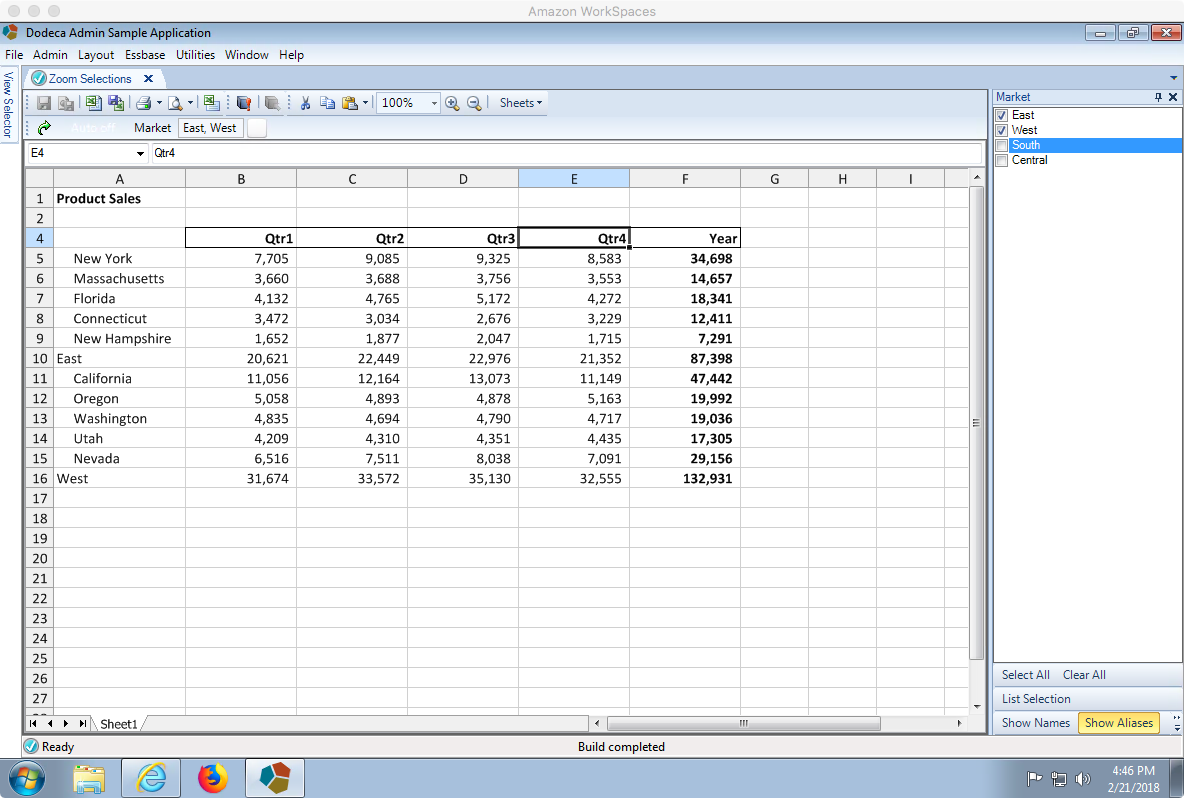
A built Dodeca view based on Sample/Basic with rows built dynamically from user selections

An example of a dynamic build based on custom selections

This example is built around the classic Sample/Basic cube that you’re likely familiar with. In terms of the user experience, we have a dynamically built selector list (on the right side, showing markets) that will use an MDX script to populate the selections directly from the outline. When the user goes to build with these selections, we will also dynamically build the report to include those selections and their children.

To briefly focus on the user experience and to some extent the developer experience, I want to really hammer the point home about the selector list. One, we’re not relegated to just showing the entire dimension and effectively sending a message to the user “Hey, go on a treasure hunt and find what you need” – we’ve completely focused the selector list to the relevant choices the user can make for this view (the upper level regions in the Market dimension). Secondly, it’s a dynamic list, so when the outline is updated, we’re automatically in sync with it, with no additional maintenance needed. This keeps things very maintainable on the development/administration side of things.

Before we dive in completely, let me point out some additional members I added to this outline to help show off this technique. Underneath each major region, there is now an input member:
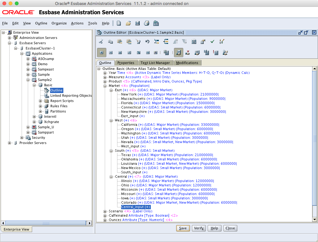
Viewing Sample/Basic outline in EAS showing that Market dimension has been augmented with level-0 input members

Outline with a twist: additional level-0 input members for regional budgeting

This is a fairly common use case where budgeting or some other activity needs to be done at a region/aggregate level, but the best practice of inputting at level-0 is being adhered to. Therefore, some budget members (East_input, West_input, etc.) are created at level-0. Some organizations don’t want to clutter up the outline and will have a “house rule” that the first or last member underneath a region might serve as the “budgeting bucket”, but my preference is for the dedicated members (you can make the case that it’s cleaner, among other things).

Setting up the template

The template for this example is pretty straightforward. The main thing we need to do are to set the named range for the Essbase data retrieve area, and then designate a starting cell for where the markets will be dynamically placed on the report.

Here’s the template with the Essbase retrieve range highlighted (note that there is a hidden row at row 3 that contains the scenario, product, and other dimensions that are essentially part of the POV):
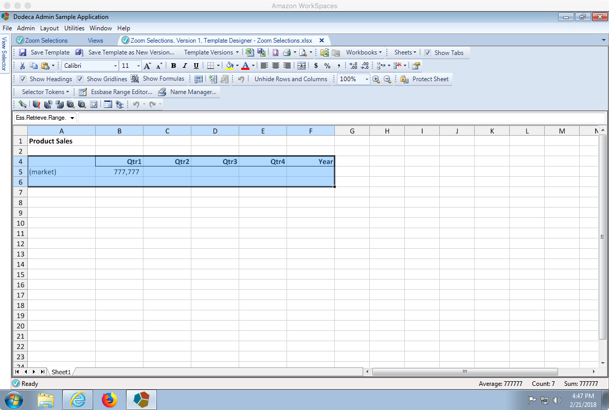
Dodeca view designer showing initial Essbase retrieve range

The nominal Essbase retrieve range in the view template

There’s nothing special about the (market) text in cell A5. It’s basically just a note to myself that it’s the location where the markets will be dynamically placed onto the template prior to the Essbase retrieve occurring. It’ll be overwritten when member names are placed in.

Next, I am going to define a named range/cell named StartCell. There’s nothing special about this particular name. This named cell will give me an easy way to refer to it from the workbook script we’ll be building in a moment. I’ll want to be able to tell the workbook script exactly where to start loading selections onto the spreadsheet:
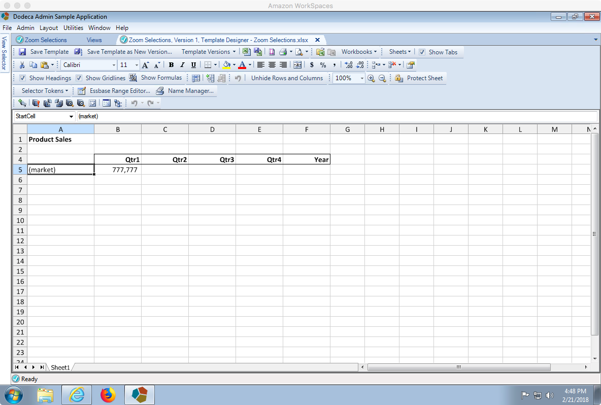
Dodeca view designer showing named StartCell

The named StartCell will serve as a starting location for a range build script

Other than that, I have just performed some incredibly light formatting on the rest of the template in terms of bolding some text, setting commas to display for numbers, and some cell borders. Once the view is functioning as expected I can go back into the template and pretty things up.

Configuring the view

With the template configured, it’s time to go set some of the options on the view itself. The view options here are fairly straightforward, with a couple of key options to set. First, notice AutoAddRetrieveSubRanges and RetrievePolicy:
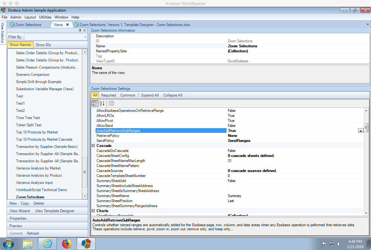
Editing options for our view in Dodeca

View options, including AutoAddRetrieveSubRanges set to true

I’ve talked about AutoAddRetrieveSubRanges before. It’s an incredibly handy option that automatically creates named ranges for various parts of the Essbase retrieve, including the row members, column members, data region, and POV header. This is really handy and powerful because we can then refer to those names in workbook scripts, as we’ll do in the last step of the workbook script in this example.

Also notice that the RetrievePolicy is set to None. This is kind of uncommon actually. Typically the RetrievePolicy is used to define how Dodeca should perform retrieves on the view – should it just retrieve the entire sheet, the specially named ranges, or nothing at all? As it turns out, this is an instance where we can simply say None, as in don’t perform the retrieve at all. This is because in this particular example, we are going to script an EssbaseZoomIn action and this will actually bring in the data from Essbase for us. So, we can turn retrieving off in the view itself.

The only other thing worth noting on the view properties is that we have a single selector set that allows multiple selections (exact selector list configuration coming up in a moment), and of course the view has a workbook script set, which we’ll get to next.

Workbook Script

As with so many views in Dodeca, a lot of the magic in showing and formatting our Essbase and other data exactly how we want and in a format most conducive to how our user wants to operate is accomplished with a workbook script. Workbook scripts let us add very sophisticated behavior to a view and activate it as needed, such as when the view is opened, built, the user submits data, or one of more than 100 other events in the view lifecycle.

Script Overview

The workbook script in this example is fairly straightforward. All of the methods occur in a single event (after the view is opened but before it’s built). Altogether we have the one event that calls the one procedure, and the one procedure has four methods that run in order. You can see all of this here:
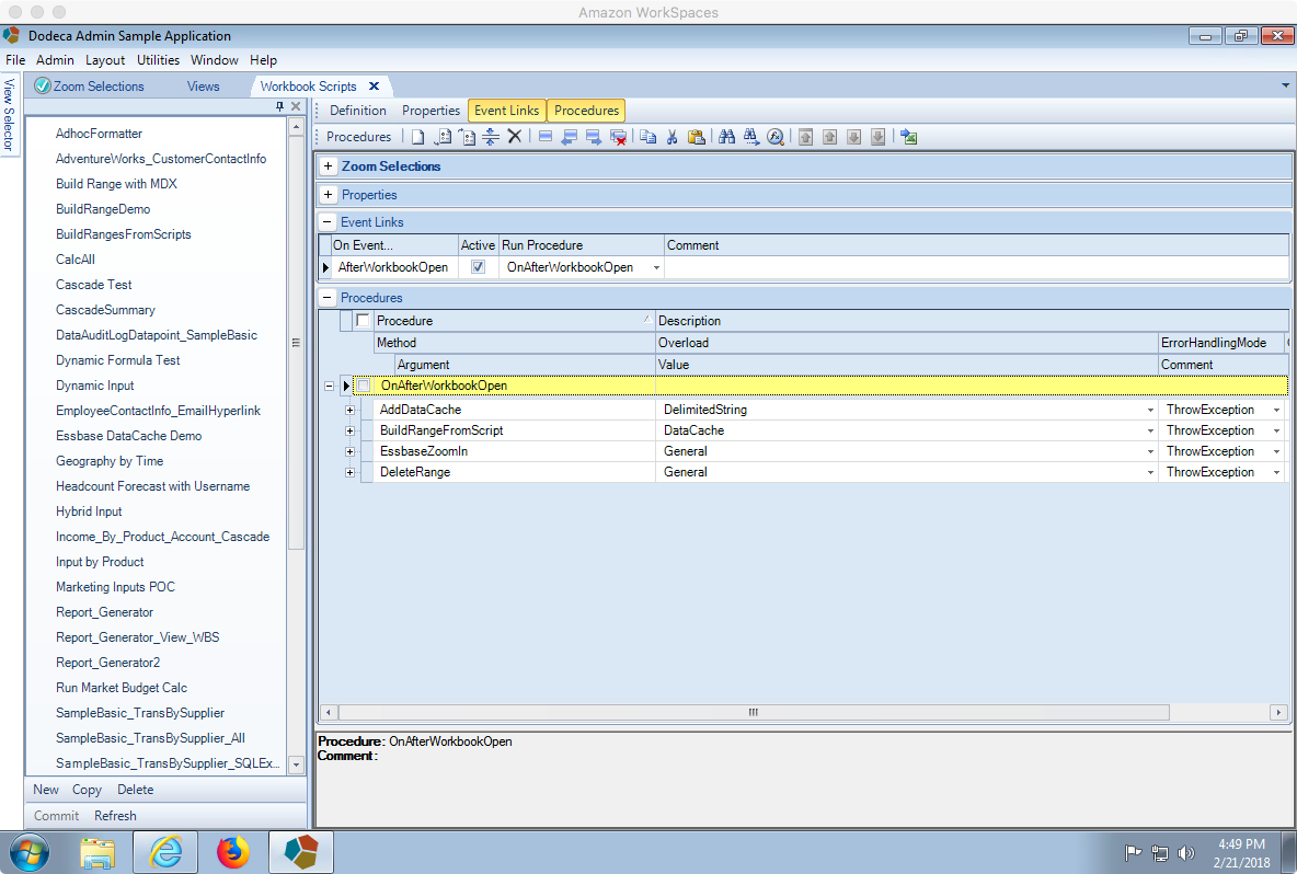
Dodeca workbook script

Overview of workbook script event links and all methods for this example

Let’s talk for a moment about the sequence of things in terms of building this view based on user inputs. The user will make one or more selections from the selector list, such as the members East and West. We need to use these as the basis of our template, so we need to somehow take those selections and place them into the spreadsheet. We’ll use the AddDataCache and BuildRangeFromScript procedures for this. Next, we’ll perform an Essbase zoom-in on these members, just as if the user had selected these members and done an zoom-in operation in Excel (except that it’s automated here). Lastly, per the needs of this view, we’ll process the zoomed-in members to remove some that we don’t want to show.

Step 1 – AddDataCache

The first thing we need to do is take the selections the user made in the selector and then process them into a list. Interestingly, this step itself don’t actually affect the template yet, it’s just putting some data into memory that we can use in the next step. I have this step configured as follows:
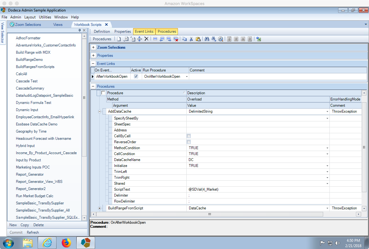
Dodeca Workbook script AddDataCache method

AddDataCache Workbook script to use selector values to build a cache/list of values to process in next step

One thing to keep in mind regarding the multiple selections the user may make is that based on how this selector list is configured, those selections will actually be concatenated together into  single string, such as “East;West“. So we’re effectively using this AddDataCache method to split the string up (using a semi-colon as the delimiter) and add it to an internal data cache named DC that will exist for the duration of this view. The ScriptText value is the text that will be split up into the data cache. We’ll use the @SDVal WBS function to get the text value of the selector with the given ID. In other words, if the selector on the view currently has East and West selected, then this function evaluates to East;West. This can be different if the selector list is specifically configured to concatenate items with something other than semi-colon, so keep that in mind.

Step 2 – BuildRangeFromScript

With the data cache successfully populated, we can now move on to the BuildRangeFromScript method to process it. We’ll specifically be using the DataCache variant (“overload”) of this method in order to process the list of items in a data cache and display those on the template. Here’s the configuration for this method:
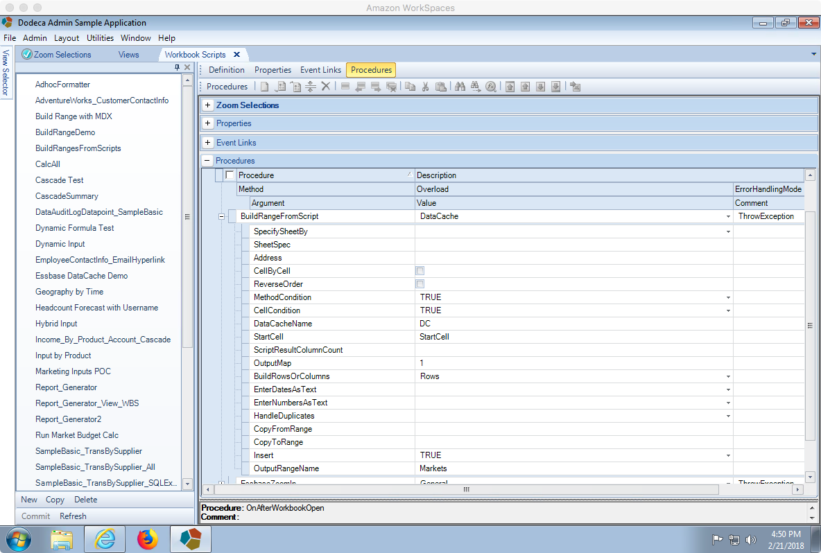
Workbook Script BuildRangeFromScript method using DataCache overload

Workbook Script BuildRangeFromScript method using DataCache overload

Generally speaking, the BuildRangeFromScript (“BRFS”) family of methods are absolute work horses are far as Dodeca views go. They are one of the most commonly used techniques to take data such as member selections, outline data, and more and arranging it on a sheet. Since we are using the DataCache variant, we have some properties specific to method that we need to set, as well as some general properties:

  • DataCacheName: the name of the data cache to process and put onto the spreadsheet somewhere. This is set to DC, the name we set in the previous step
  • StartCell: this is the starting location we set in the template by setting its name. Technically we could make an absolute cell reference here but the best practice is to use a named range, as improves maintenance and readability
  • OutputMap: the output map probably warrants an article of its own, but for now just set this to 1, which will work just fine in this “single column” example.
  • BuildRowsOrColumns: the BRFS is flexible enough to lay things out along rows or columns. Set this to Rows because this is what we want to build.
  • Insert: set to True. By setting this to true, it means that when each item from the data cache is being added to the spreadsheet, it will technically be added by inserting a new row and adding it, as opposed to just just dumping them on the spreadsheet. This is useful for a couple of reasons. The thing that’s most important to us here is that it’ll cause the area covered by Ess.Retrieve.Range.1 to be expanded as the member names are inserted, so we’ll still be able to do a normal Essbase retrieve afterward.
  • OutputRangeName: once the BRFS runs, it can optionally create a named range around all of the data that was output onto the spreadsheet. We’ll set this to Markets because having a named range will make our next step very simple

Step 3 – EssbaseZoomIn

At this point we should have an Essbase retrieve range that is populated with the selections that the user made (a screenshot of this intermediate step will be shown in the next section when we walk through the workbook script step by step). With those members now properly laid out, we can now perform the zoom-in step on the entire range using the EssbaseZoomIn method. This is where the OutputRangeName from the previous step comes into play and makes things easy for us.

Here’s the configuration for this method:
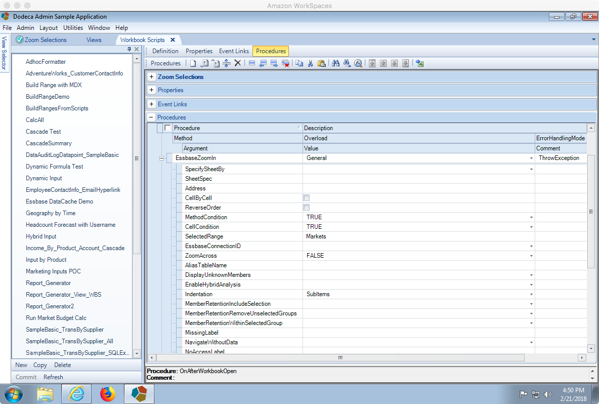
WBS to perform an Essbase zoom in

WBS to perform an Essbase zoom in

There are a couple of properties that didn’t show in the previous screenshot, here’s the rest:
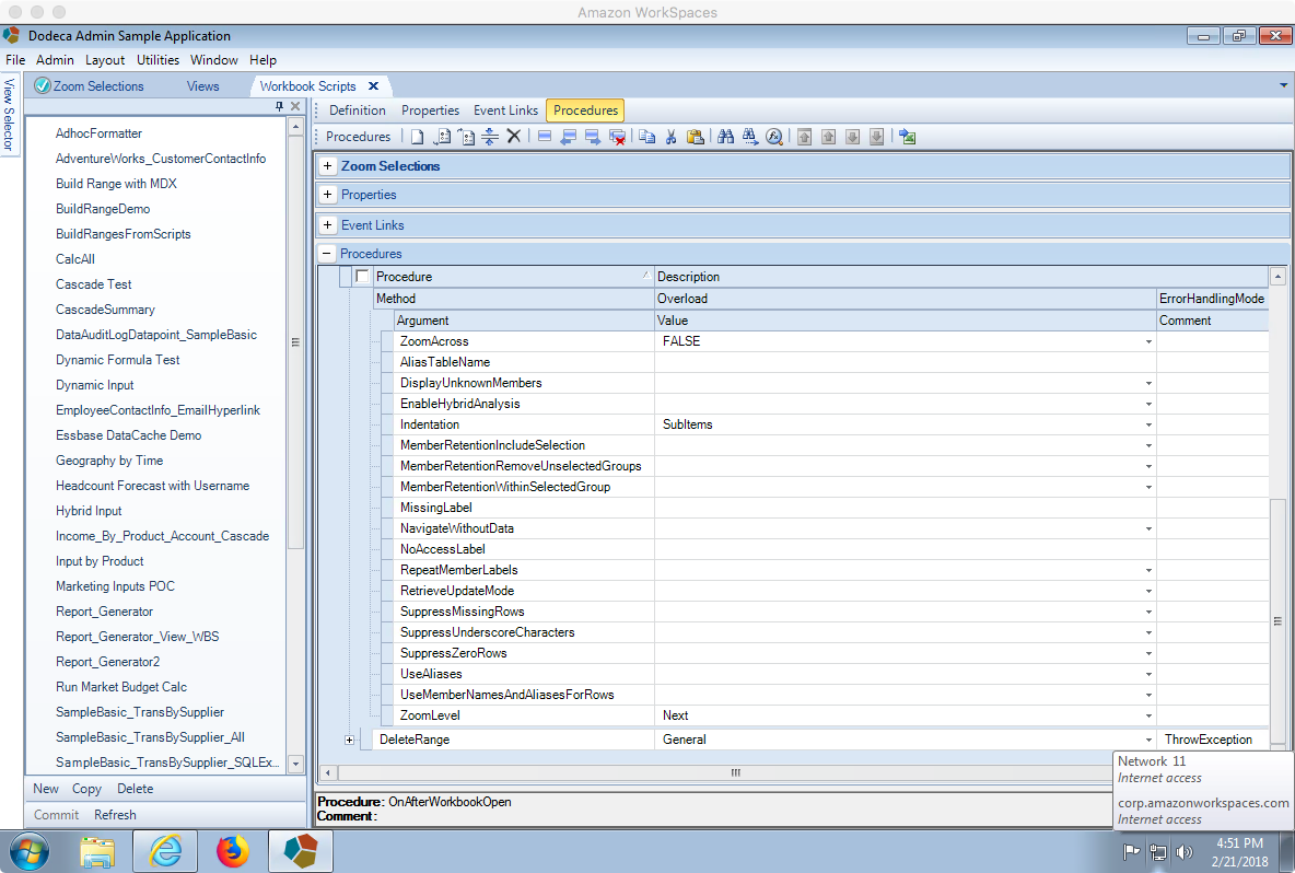
The rest of the zoom in method, showing a zoom level of Next

The key properties here are the following:

  • SelectedRange: a range name to zoom in on. We’ll use the range that was automatically created for us in the previous step, so it’s effectively like we’re performing a zoom-in on multiple items. I wanted to put a little extra emphasis on this because probably the much more common zoom operation is to just zoom-in (such as double clicking) on a single item.
  • Indentation: this isn’t really a critical setting in this context, but I thought it’d be nice to just use the indentation setting to show that this is, indeed, almost exactly like performing a normal zoom operation, including how the resulting data should be formatted (in terms of classic ad hoc options).
  • ZoomLevel: Next. As with the previous setting, we have immense control over the exact mechanics of the zoom, including what level to zoom to, which in this case should be next (as opposed to bottom or siblings).

Step 4 – DeleteRange

The last step in the overall procedure is to remove some items that we don’t want to show. We can use the DeleteRange method for this purpose. This really isn’t anything to do with Essbase per se, just a normal spreadsheet operation. Here’s the configuration:
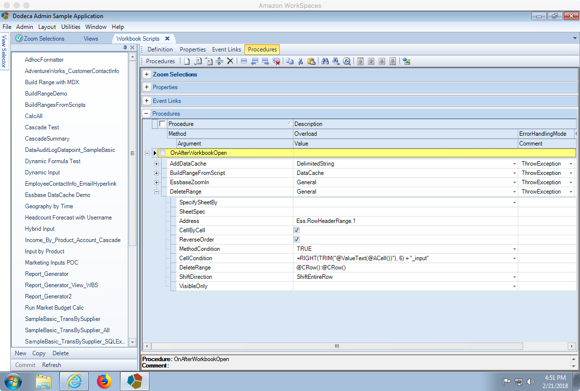
DeleteRange workbook script method

Workbook script to delete rows meeting certain criteria (acts as a filter)

There are a lot of interesting things going on here that might appear complicated but are quite logical. Let’s step through the settings on this procedure step by step to get a full sense of what’s going on:

  • Address: this is a standard WBS setting that defines the specific range that the procedure will operate on. Since we want to filter rows here, we can use the range that was created for us automatically on the Essbase retrieve that outlines the range containing the rows. So to be clear, this range will contain all of the members from the Market dimension that are on the spreadsheet, including after the results of the previous zoom-in operation.
  • CellByCell: when turned on, this option means that the procedure will be evaluated for each cell in the Address.
  • ReverseOrder: this tells Dodeca to evaluate the contents of the range in reverse order (i.e. from the bottom up). This option is almost always used – and necessary – when deleting rows/columns from a sheet, as otherwise the delete operation wouldn’t work as expected.
  • CellCondition: this is probably the most sophisticated aspect of the entire procedure. This is where we can specify a condition that must evaluate to True in order for the procedure to be executed for the current cell. In other words, for our purposes here, the procedure cell condition is evaluated for every cell in the range and when it’s true, then the actual operation (a row deletion) will occur.

The cell condition here is a combination of normal Excel formulae and workbook script functions. Here’s the full formula:


=RIGHT(TRIM("@ValueText(@ACell())"), 6) = "_input"

The Dodeca interpretation of this formula would be the following: if the rightmost 6 characters of the trimmed contents of the active cell are equivalent to the text "_input", then delete the range as specified in the DeleteRange property. So, we we have two Excel functions (RIGHT, TRIM) and we have two Dodeca WBS functions (@ValueText, @ACell). The @ACell() function evaluates to the address of the current cell being evaluated. Combined with the @ValueText() function, we get the contents of the active cell, such as East or East_input or whatever it is.

In case you’re not familiar with this sort of boolean (true/false) logic, please note that this example is exactly equivalent to the longer form that uses an actual Excel IF statement:


=IF(RIGHT(TRIM("@ValueText(@ACell())"), 6) = "_input", TRUE, FALSE)

Lastly, we don’t strictly need the TRIM function here but it doesn’t hurt. If we were looking at the left side of the cell contents rather than the right side, then we would almost definitely want to use TRIM because the cell contents might have spaces on them from the Essbase zoom-in indentation setting.

Let’s move through the rest of the settings in this DeleteRange method:

  • DeleteRange: this property (which happens to share its name with the procedure itself) specifies what to actually delete when the previous CellCondition evaluates to True. As with the previous property, Dodeca functions will help out immensely here, particularly the @CRow() function, which evaluates to the current row of the cell being processed. The syntax @CRow():@CRow() might look a little funky, but it is how we can refer to an entire row in Excel. For instance, if row 4 of the sheet is currently being evaluated, then this property evaluates to 4:4, which is a valid range that will be deleted.
  • ShiftDirection: currently set to ShiftEntireRow, which is more or less just like telling Excel how to shift cells around when performing the delete (as opposed to ShiftLeft, ShiftUp, or ShiftEntireColumn).

Selector List Configuration

I mentioned at the start of this post that one of the things Dodeca brings to the table in terms of the user experience is the ability to tailor the selections that a user can choose from. These selections can be populated in several ways: a pre-defined list, an Essbase report script, SQL, an MDX script, and more. A simple MDX script will fit the bill quite nicely here. The selector list configuration is pretty standard:
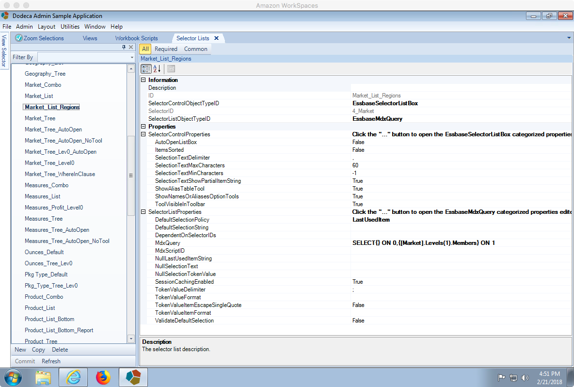
Setting options for the Market selector list

Setting options for the Market selector list

Most of this is pretty default – the object type is an EssbaseMdxQuery, the DefaultSelectionPolicy is LastUsedItem (meaning to pre-select the last item the user used on this view, if any), and then there is the MDX query (MdxQuery setting) itself, which can be edited directly in Dodeca’s syntax-highlighting editor:
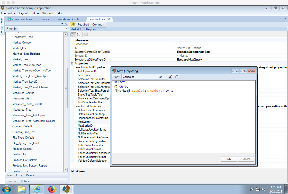
Editing MDX script that returns level 1 members from Market dimension

MDX script to return level 1 members from Market dimension (West, East, South, etc.)

The script to generate a list of all of the Level-1 members from the Market dimension can be written pretty simply:


SELECT
{} ON 0,
{[Market].Levels(1).Members} ON 1

As applied to the Sample/Basic outline, this generates a list containing East, West, South, and Central. If we add new level-1 members to the outline, they’ll show up automatically. There are other ways we might choose to formulate this query, by the way. For example, it might make more sense to write the query such that it just pulls the children of the Market member, rather than the members from level 1. It depends on the particular nuances of the dimension/outline, but this will work fine for now.

Building & Stepping the View

We’ve covered a lot of ground to get to this point: the template, view settings, selector configuration, MDX script, workbook scripts, and more. With everything in place it’s now time to run the view. Rather than just showing the built view and calling it a day, I want to do something a little more involved, so you can get a sense of the sequence and operation of the workbook script. In order to step the workbook script procedure by procedure, we need to make sure that debugging is turned on for the script. This is set in the main configuration of the script, via the DebugMode setting:
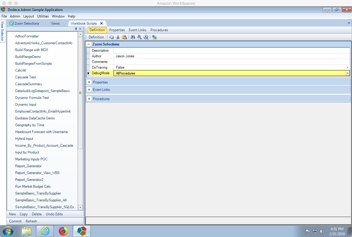
Turning on DebugMode for a workbook script

Turning DebugMode on in our Workbook Script so we can view it step by step

Now when we launch the view (as if we were a user running it), the workbook script debugger will pop up:
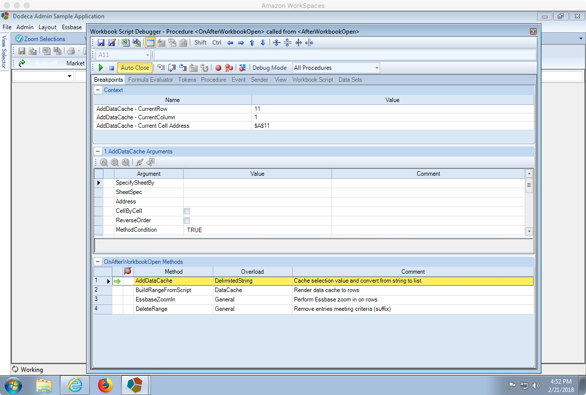
Watching WBS execute step by step: running first step and turning on displaying the view build in real-time

One thing we can do to make the step-by-step viewing process easier to interpret is to show the template in real time. We can do this by unselecting the Cover View button, which is the fifth button in the first toolbar of this debugger window. Upon uncovering the template and stepping to the next procedure, we’ll see this:
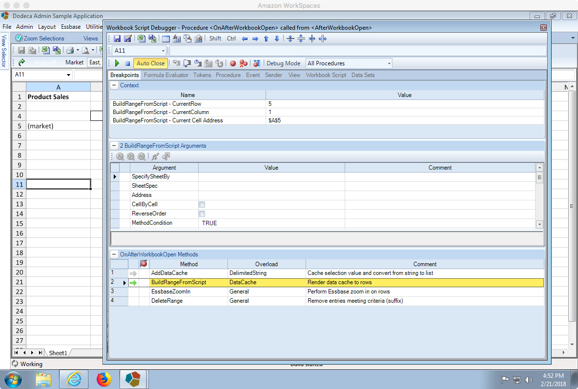
Watching the WBS execute step by step, prior to build range step

The button to move to the next step is just to the right of the “Auto Close” button. We have various programming-like debugging steps, but the only one we need here is to step to the next procedure. At this point, the AddDataCache method has already executed. As discussed above, though, it doesn’t actually have any physical effect on the template. BuildRangeFromScript is going to affect things, though:
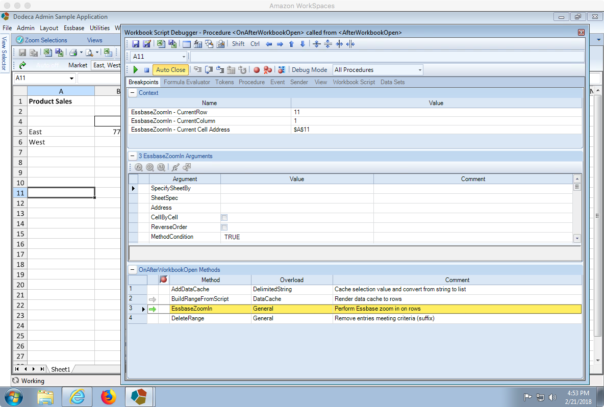
Viewing template after BuildRangeFromScript has executed

Notice that the selections from the selector (East & West) have now been placed in column A right where the StartCell was set. Now we can perform the Essbase zoom-in:
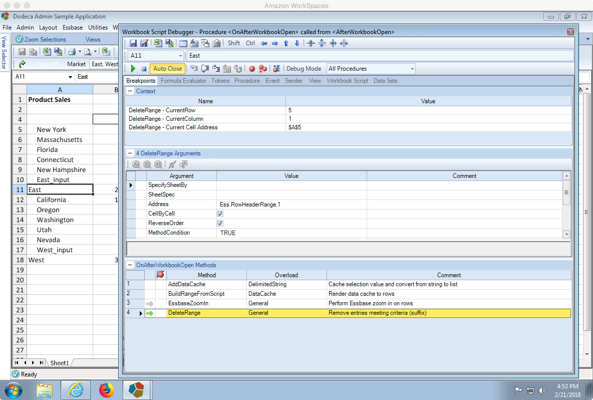
Viewing template after EssbaseZoomIn step has executed

Everything looks good so far. As expected, the extraneous “_input” members that are part of the dimension were also brought in and put on the spreadsheet. To finish things off, we’ll continue by running the delete step, which upon completion will cause the workbook script debugger window to automatically close, leaving us with just our view:
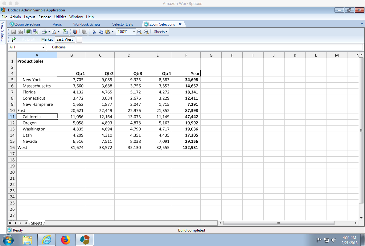
Viewing template after the DeleteRange step has executed (_input members are gone)

Just for fun, let’s take a look at the range that Dodeca automatically created for the row members of the Essbase retrieve range:
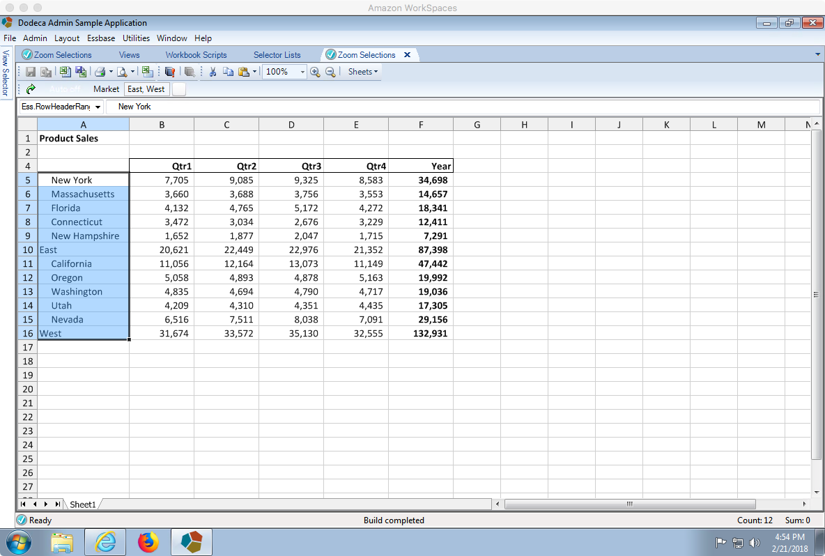
Checking out the automatic Ess.RodHeaderRange.1 named range

As with the BuildRangeFromScript expanding one of our named ranges earlier, the opposite is true when we go to delete: the range shrank, just as it would if we had deleted the row in Excel.

Summary

We covered a lot of ground here: data caches, dynamic build ranges, workbook script, MDX selector lists, debugging, and more. I hope you found this walkthrough insightful and how Dodeca can be used to complement Essbase and operationalize your data in the exact way that your users want to see and interact with it.

PBCS Scripting with Groovy using the PBJ REST API Library

I was talking to a colleague the other day that wants to do some scripting with PBCS using Groovy. Of course, since PBCS has a REST API, we can do scripting with pretty much any modern language. There are even some excellent examples of scripting with PBCS using Groovy out there.

However, since Groovy runs on the JVM (Java Virtual Machine), we can actually leverage any existing Java library that we want to – including the already existing PBJ library that provides a super clean domain specific language for working with PBCS via its REST API. To make things nice and simple, PBJ can even be packaged as an “uber jar” – a self-contained JAR that contains all of its dependency JARs. This can make things a little simpler to manage, especially in cases where PBJ is used in places like ODI.

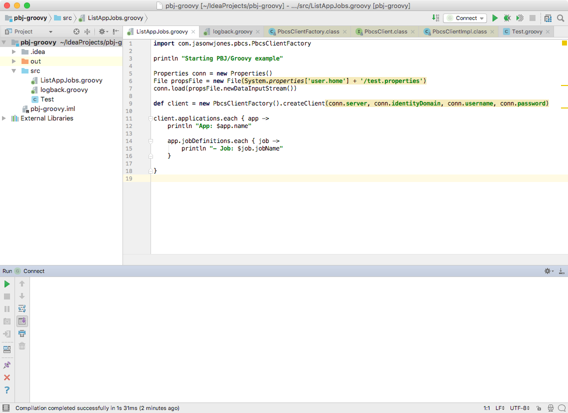
For this example I’m going to take the PBJ library uber jar, add it to a new Groovy project (in the IntelliJ IDE), then write some code to connect, fetch the list of applications, then iterate over those and print out the list of jobs in each application.

I’ll just jump right into the existing project I have so we can get our bearings. The following screenshot shows the full script in the IDE:

IDE screenshot of Groovy file using PBJ PBCS library to connect to PBCS and get list of jobs in all apps

Code listing for a simple Groovy script that connects to PBCS via the PBJ library, lists the apps and all of the jobs in the apps

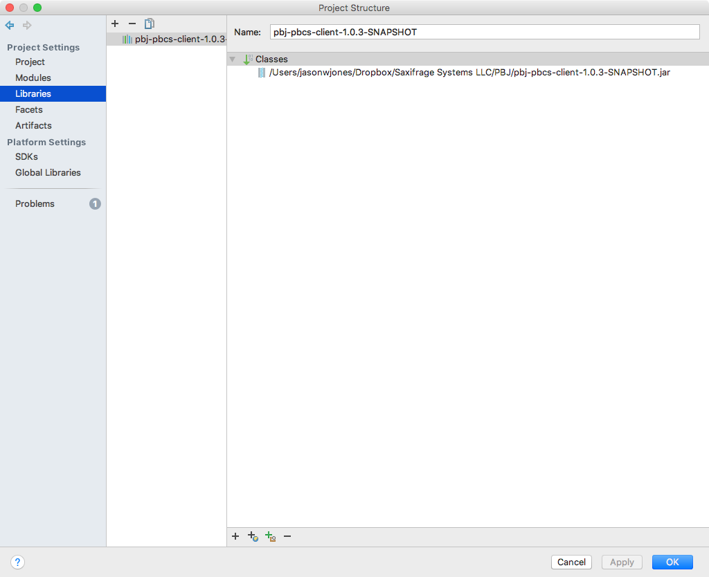
The first thing we need to do is actually reconfigure the project to include the PBJ library JAR. We can do this in the project settings by adding the library:

IntelliJ Project Structure window for managing referenced libraries

The PBJ “über JAR” is included in the Project Structure Libraries list

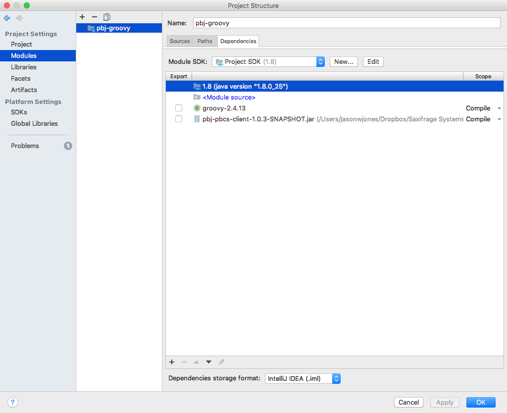
Note that the path doesn’t really matter. You can obtain/build the uber JAR file by going to the PBJ GitHub page, cloning the repository, then following the instructions from the README file on how to package a jar this way. We can review the list of referenced libraries on the Modules tab for good measure:

IntelliJ Project Structure window showing Modules for Groovy test script

Upon adding the PBJ jar to our project in the Libraries tab, it shows up in the Modules configuration as well

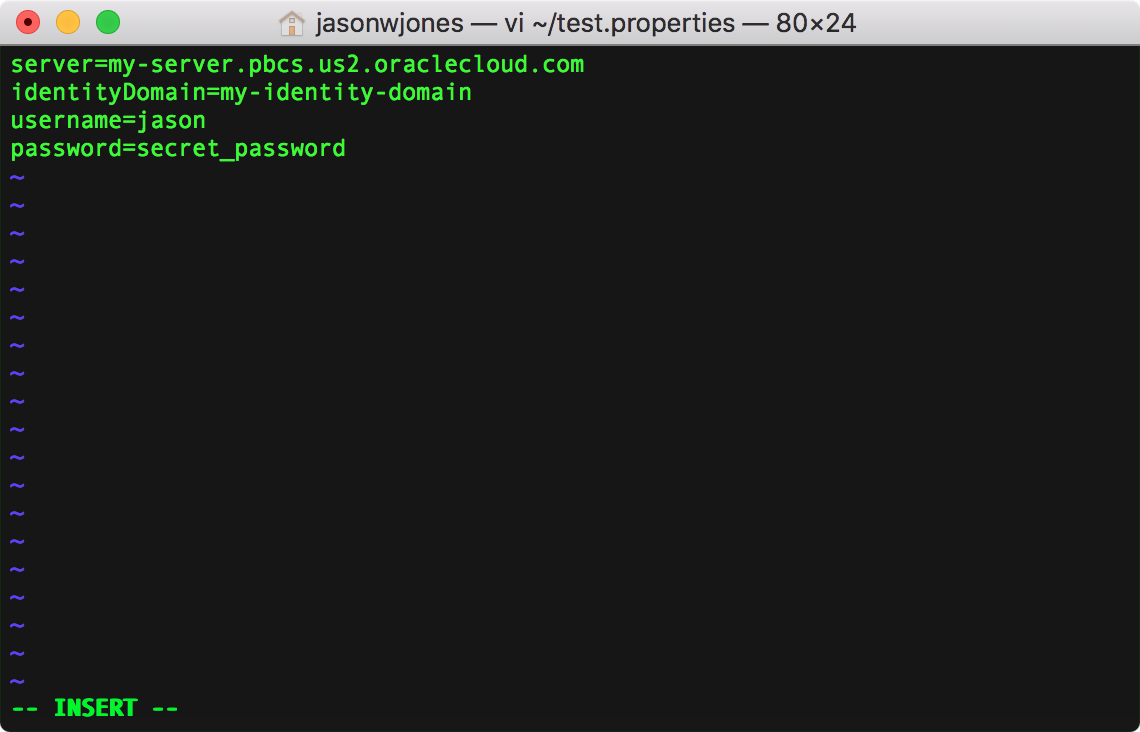
Now we’ll turn our attention back to the code itself. You may notice one the first lines references a file in my user folder. This contents of this file (anonymized of course) look like the following:

Example format of properties file containing connection settings for the test script

Simple configuration file in user home folder that contains the connection parameters (server, identity domain, username, and password)

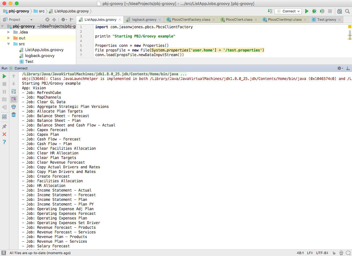
Upon successfully configuring the properties file and running the script, I can check out the output:

IntelliJ IDE showing output from the Groovy test script

The output of running our job to list the apps and their respective jobs using the PBJ API

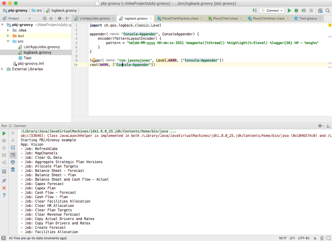
Hey hey, things worked perfectly! For completeness I want to draw some attention to the fact that there was no logging output when we ran the script. That’s because I had configured it (via a logback.groovy configuration file) to only print messages that were warnings or worse. There weren’t any, so there was no logging output. Here’s the logging specification:

Editing the logging configuration for our sample script

PBJ’s logging framework allows for specifying a configuration file as a Groovy script itself

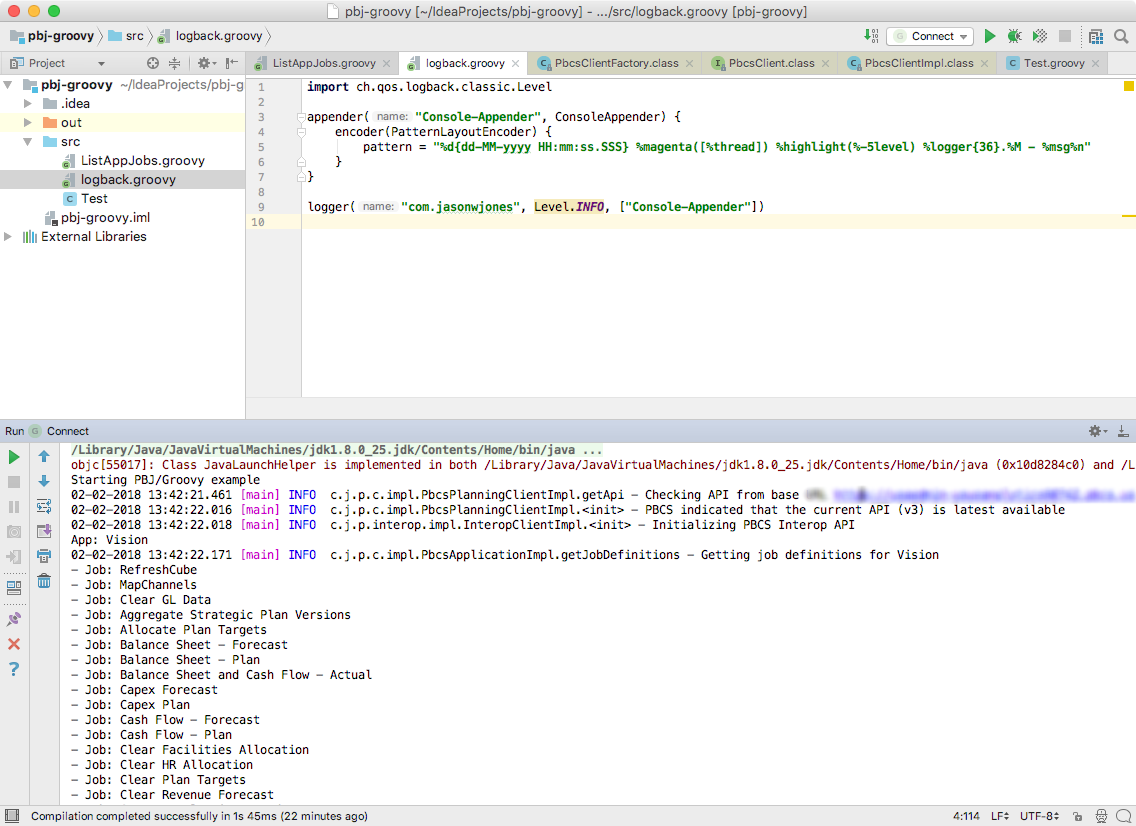
Let’s drop the threshold down to INFO (so that info, warning, error, and higher will print) and run it again. We’ll see that the low-level logging messages from the library now print out:

Script output of apps and jobs after editing logging settings to show messages

Script output including informational logging messages

Note the colored INFO log messages in the output. These are messages that are built in to the programming of the PBJ library itself and will often be useful to help diagnose issues or otherwise see what’s going on.

The Code

The code itself is pretty simple. In fact, most of it is just loading a the properties file and using it to setup the connection using PBJ’s PbcsClientFactory object (which is the starting point for using PBJ). Whereas in Java we might typically use a for loop to iterate something, Groovy provides some syntactic sugar to iterate using each. So in the below example we just iterate the apps, and then iterate each job definition in each app.


import com.jasonwjones.pbcs.PbcsClientFactory

println "Starting PBJ/Groovy example"

Properties conn = new Properties()
File propsFile = new File(System.properties['user.home'] + '/test.properties')
conn.load(propsFile.newDataInputStream())

def client = new PbcsClientFactory().createClient(conn.server, conn.identityDomain, conn.username, conn.password)

client.applications.each { app ->
    println "App: $app.name"

    app.jobDefinitions.each { job ->
        println "- Job: $job.jobName"
    }

}

Benefits of this Approach

I really like this approach for several reasons. One, since an existing library has already concerned itself with communicating with the REST API and it’s possible to leverage that library in Groovy, why not? The PBJ library is an open source library that covers most of the PBCS REST API, and by using it we get to stand on its shoulders and void lots of boilerplate code processing in Groovy, thus rendering us able to do high-level things with an absolute minimum of code.

Happy New Year &#038; Best Posts of 2017

My goodness – has another year gone by already? 2017 was busy, to say the least: trips/presentations/booths at Kscope17, Collaborate, and Oracle Openworld, new releases of Dodeca, the Dodeca Essbase Add-in for Excel, Drillbridge, the Outline Extractor, an upgrade to Oracle ACE status, lots of internal development going on, and more.

Speaking of Kscope, did you submit an abstract for Kscope18 yet? The submission deadline is very quickly approaching.

In any case, I covered a lot of ground on the blog this year, and as with last year, I thought it would be fun to take a look at the best and most popular posts of 2017!

Most Popular Posts

JDBC and JNDI Connections Compared

Oddly enough, the most popular post of 2017 was an article I wrote comparing, contrasting, and explaining the differences between JDBC and JNDI connections, with an emphasis on how it pertains to configuring Dodeca’s middle-tier components. I have to imagine that this actually garnered some non-Essbase/Hyperion attention since JNDI configuration can be a bit of a dark art and tough to figure out, especially for people that are only used to JDBC.

I’m either sad or happy that this ultra-technical post was the number one post of the year. I’m not sure yet.

Hacking the Essbase Java API to Run Application Calcs

In second place is another ultra-technical and almost entirely useless post in the literal sense of the word about how you can run old-school application-level calcs on an Essbase cube, even though EAS and the Java API conspire to make it seem like it was never actually a thing.

Essbase Renegade Members Revisited

Whatever happened to renegade members and the dream of being able to shovel almost imaginable garbage into a cube that will still tie out at the top of the house? I dig into the diminutive renegade member feature and give it some love.

Improvements to the Next Generation Outline Extractor

Hey, finally something useful. The next most popular post was about a raft of improvements and fixes to everyone’s favorite free tool, the outline extractor. The outline extractor continues to be a very popular download and possibly the most downloaded tool of its kind in the Essbase ecosystem. Some fun things are in store for this tool in 2018.

Essterm: the terminal based ad hoc client for Essbase

Rounding out the list of popular posts was my post detailing my latest flight of fancy and dubiously useful tool: Essterm a terminal based client for Essbase. Look, no one said that Essbase was sexy. So why not go full 80’s-neon-lime-green text-in the terminal with it? My favorite quote of all was from Peter Nitschke: “I thought it was fake until l realized that it would have been more work for you to fake it than to actually make it.”

Than you, Pete, I’ll take that as a compliment.

Honorable Mention

In the top trafficked pages for the entire website, a couple of other URLs jumped out in addition to the posts above. Both the category and tag URLs for MaxL were on the top 10 list. In other words, people are still really needing and hungry for MaxL content, need help with it, and doing things with it. This makes sense, of course. But it’s still interesting…

Honorable Mention – Older Posts

Also in the top 10 list of popular URLs were various old and older posts that are getting a lot of attention, interestingly enough. In order: a Do This/Not That post on Scenario dynamic calcs with regard to the previous year, a very old post on post on how to copy an Essbase application from one server to another (this is pre-LCM, maybe I should write an update…), some deeply researched analysis on a “nefarious” ODI issue that burns sequence values when using the MERGE update strategy (ah, memories), and a super throwback Essbase optimization story where I did a soup-to-nuts refactoring of a critical automation system for a Fortune 50 company to cut processing time down from 6 hours to 37 seconds (pre SSD, thankyouverymuch).

Here’s to 2018

May the year 2018 be even better than 2017 – I look forward again to seeing and talking with all of my esteemed Essbase colleagues in the upcoming year as we talk about all things Essbase, cloud, drill-through, spreadsheets, and more.

Evolution of Essbase: new URL-based drill-through showed up in 11.1.1.3

Continuing on with the idea of getting insight into the Essbase feature set over time, as viewed through the lens of its Essbase Java API evolution, you can quite clearly see that the open/URL-style drill-through (as opposed to classic LRO-based drill-through) showed up in version 11.1.1.3, which in fact is pretty much the only thing that seemed to get added to this particular release, Java API-wise, along with some ancillary drill-through methods/functionality in some related classes.

More near to my heart: this is the exact functionality that paved the way for Drillbridge! Although it wasn’t available as a feature on day 1, subsequent versions of Drillbridge gained the ability to automatically deploy drill-through definitions to a given cube, and it uses exactly these API methods to accomplish it.

Drillbridge as drill-through solution with CSV data and replacing Access

An interesting use-case has come up with Drillbridge recently where drill-through is currently being “handled” with an Access database. I put the quotes around handled because the current solution requires the user to look at the current POV and then go fetch the corresponding data from an Access database. You might be thinking that this setup is horribly sub-optimal, but I wouldn’t characterize it as such. In my career on all sides of Hyperion – a developer, a consultant, and software developer – I have seen this pattern (particularly those involving Access) pop up again and again.

Access is often (perhaps all too often) the glue that binds finance solutions together, particularly in cases like this involving drill-through. It’s cheap, you can use it on the network simply by dropping the file onto a share drive, it gives you a quick and dirty GUI, and more. Many EPM projects I have been on involve many deliverables, often including drill-through. And all too often those projects had to cut it due to budget and time constraints. And if it gets cut, sure, finance might have to do the “quick and dirty” option like this with Access.

Now, the request du jour: use Drillbridge to quickly implement true drill-through, where the data currently resides in an Access database? A couple of options come to mind:

  • JDBC to ODBC data bridge to access current Access database
  • Export Access data to relational database
  • Export to CSV and access via JDBC CSV reader
  • Read CSV dynamically using Drillbridge’s embedded database

I won’t bore you with an exhaustive discussion of the pros and cons of these options, but I will say that the JDBC/ODBC bridge was a non-starter from the get-go (for me), mostly because I looked into it for another project years ago and the general consensus from Sun/Oracle was a) don’t do that [anymore] and b) performance is not too great. Regarding exporting Access to a relational database, yes that is more towards the ideal configuration, but if that were an easy/quick option in this case, we probably wouldn’t be on Access already (i.e., for whatever reason, finance didn’t have the time/patience to have the IT department stand up and manage a relational database, to say nothing of maintenance, ETL, and other things). Next, while there are a handful of JDBC CSV readers, they seem to have their quirks and various unsupported features, and hey, as it turns out, Drillbridge’s embedded database actually ships with a pretty capable CSV reading capability that let’s us essentially treat CSV files as tables, so that sounds perfect, and bonus: no additional JDBC drivers to ship. So let’s focus on that option and how to set it up!

Getting Started

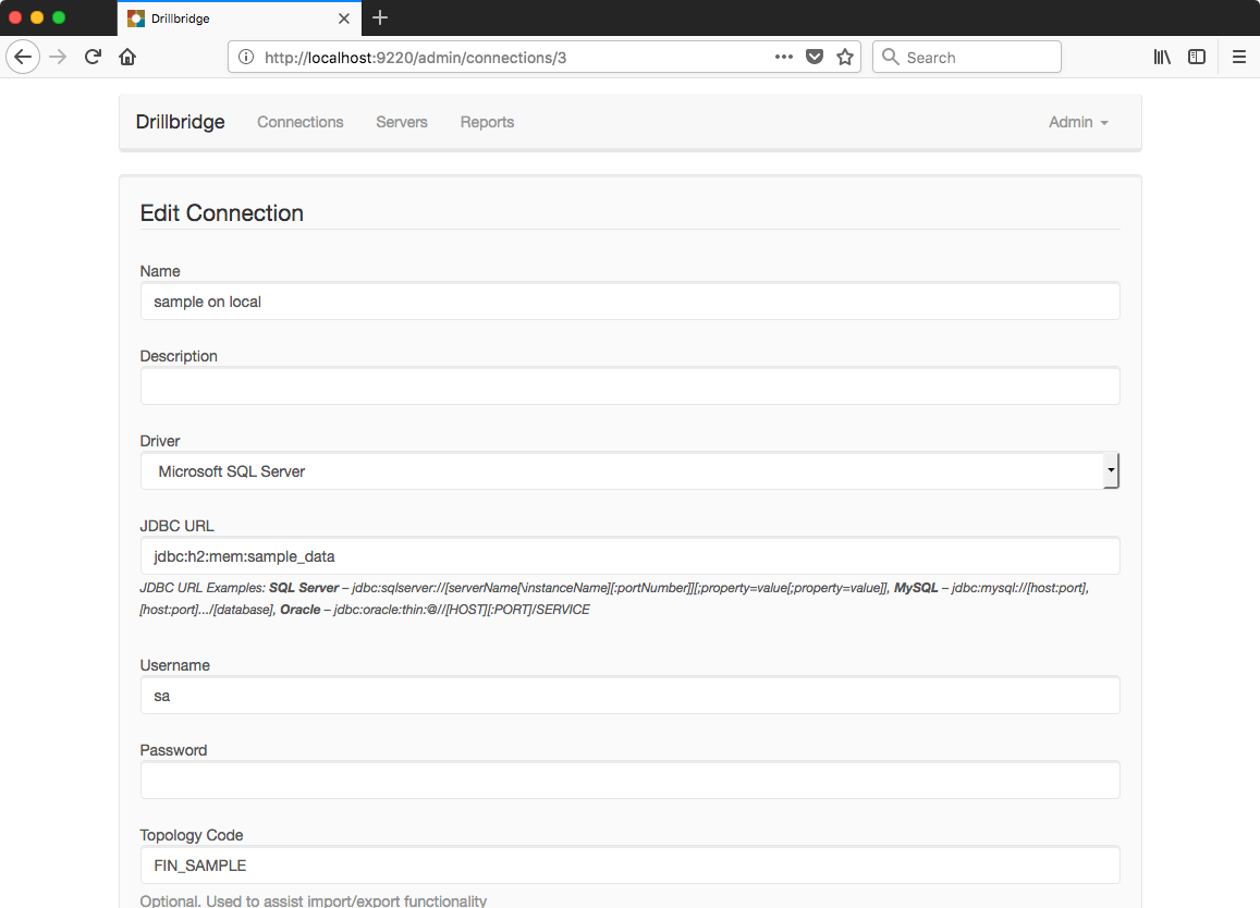
Access Drillbridge and configure a new connection:

Setting up H2 in-memory JDBC connection

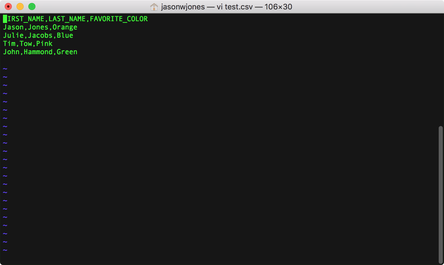
You may notice that the Driver type says Microsoft SQL Server – it’s not actually, if you look at the JDBC URL you can see that we are specifying a JDBC URL for the H2 database. H2 ships with and is used by Drillbridge; we can setup a new instance totally in memory by using the special URL: jdbc:h2:mem:sample_data. You can replace sample_data with whatever you want. Drillbridge will inspect this JDBC URL and use the proper driver, irrespective of what the Driver setting says. That’s actually all the config we need with regard to the data source. Next, let’s consider a simple CSV text file that we’ll want to query:

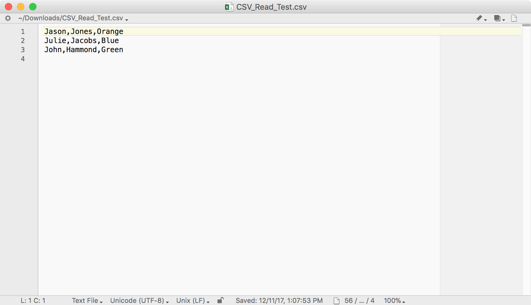
Simple CSV file with column headers (FIRST_NAME, LAST_NAME, FAVORITE_COLOR)

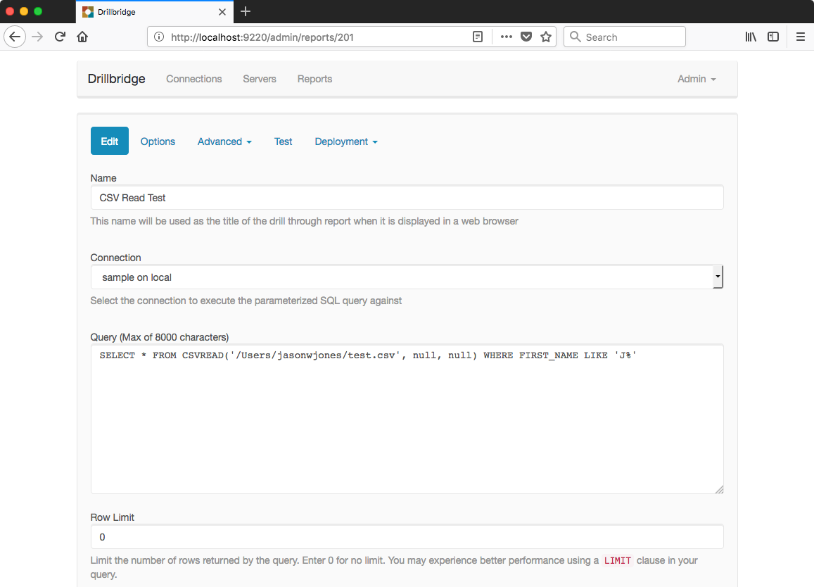
Note that the first row contains the column titles/field names. This isn’t strictly required but it’ll make life much simpler in a moment (because we can treat those as column names in our query). Now we can head over to the new report definition. To make this work, we’ll use H2’s built-in CSVREAD functionality. As a pedantic matter, note that I said functionality, not function. That’s because we’re treating the CSV file basically as a totally dynamic table, as opposed to having to import it upfront, all at once.

Defining the Drillbridge query to read from CSV file (CSVREAD), also with LIKE clause

You may further notice that I put a WHERE clause in, just to show that totally normal SQL filtering works exactly how we expect it to. For reference, here’s the full query: SELECT * FROM CSVREAD('test.csv', null, null) WHERE FIRST_NAME LIKE 'J%'. I’m running this just from my laptop which is why you usee the full file name in the screenshot pointing to a file in my home directory, but in principle, any file that the Drillbridge Java process can read should work just fine. Even, theoretically, a file off of a network share (although performance would go down a little bit).

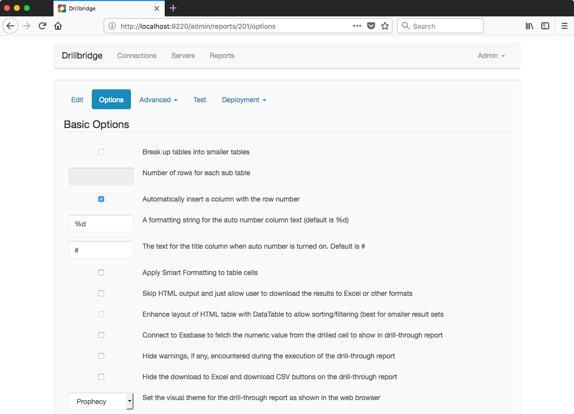
Next I’ll set a few basic report options. I don’t really need to set these to make things work, but it shows off some of the flexibility that Drillbridge has in terms of formatting the output nicely. I’d like Drillbridge to slice in a new column with an auto-generated row number, title this column with “#”, and use the modern “Prophecy” theme that makes Drillbridge blend in very nicely with Oracle’s livery, as it were:

Setting some options on the output

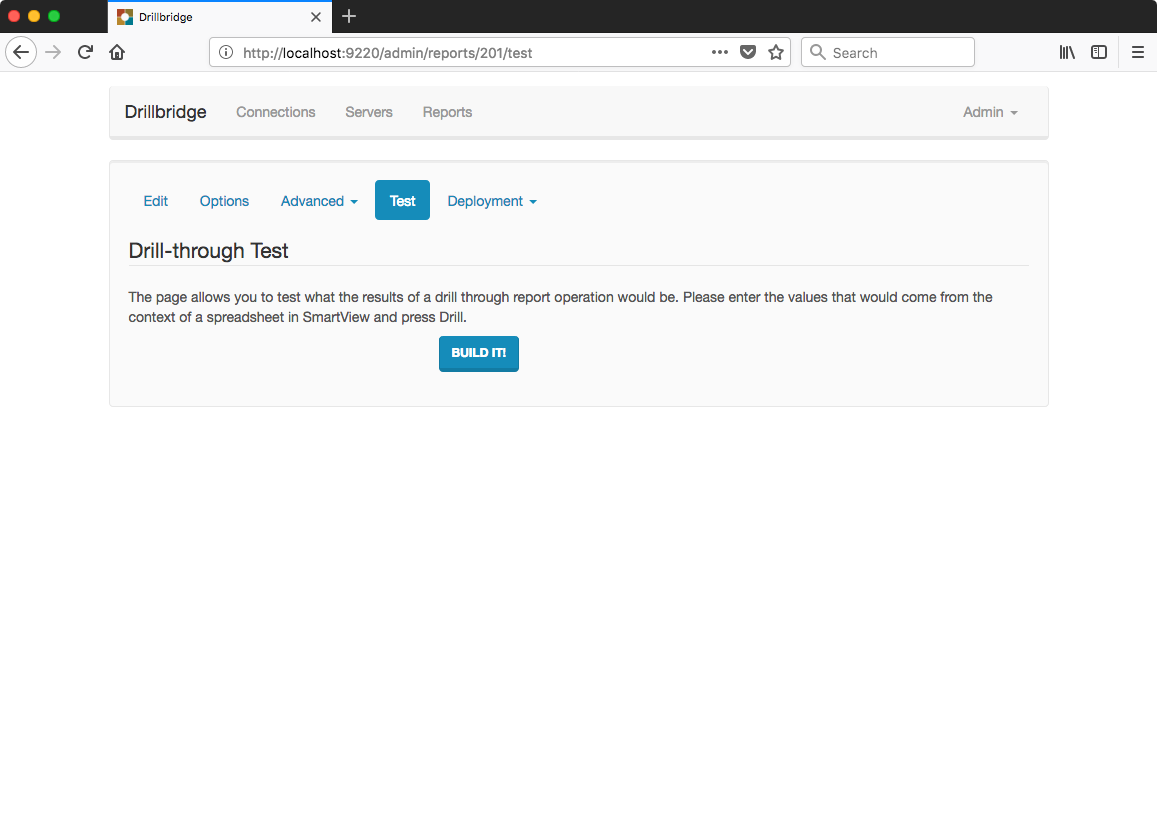
Now to save the report definition and proceed to test it:

Test page

There are no tokens in this test (although they work just fine as always), so we can just press the Build It button and test things out:

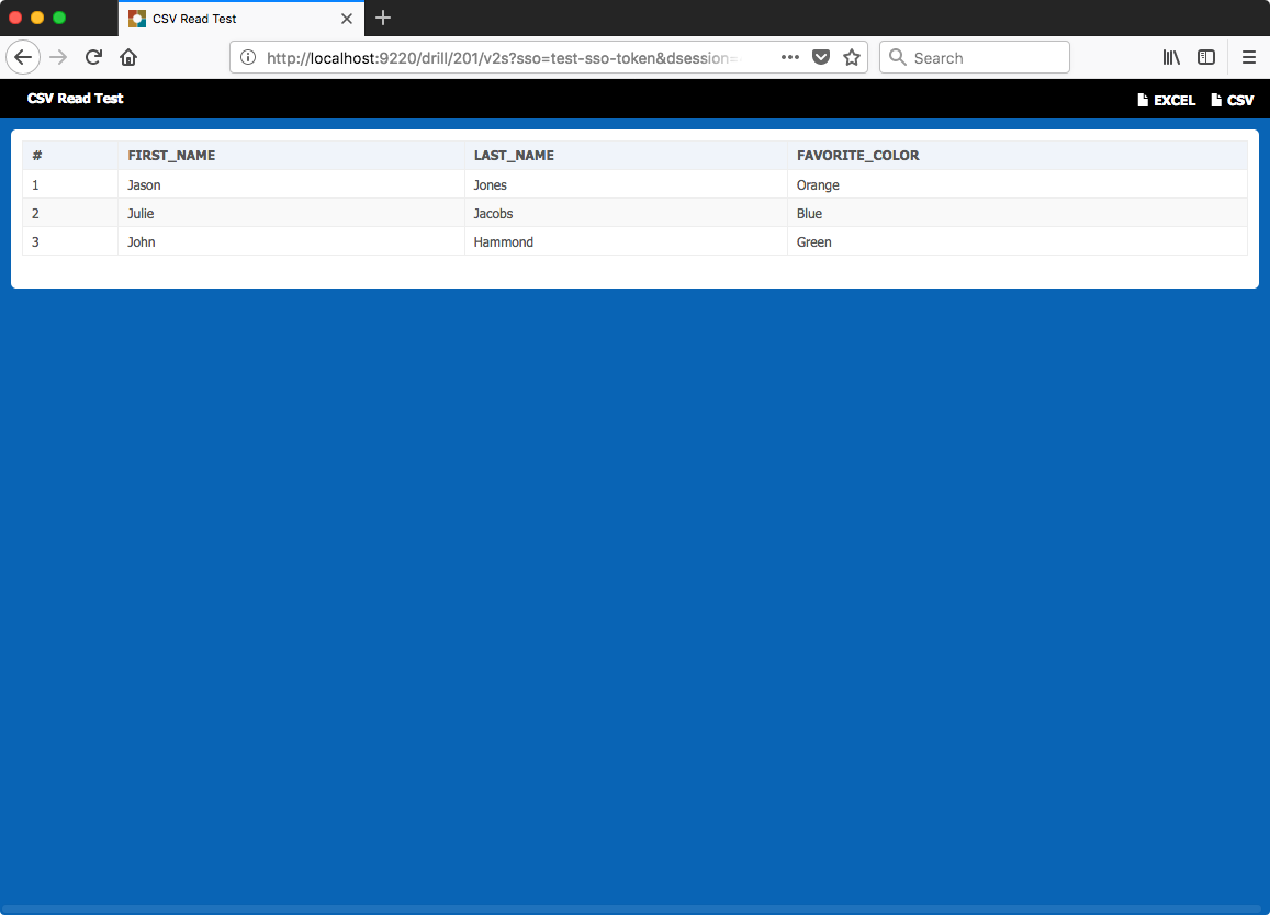
Result of testing

Sure enough, things work exactly as expected, and the data was filtered perfectly as well (in this case, only showing rows where the FIRST_NAME starts with the letter J). And just for completeness, let’s download as CSV to test what we get:

Output when downloading to CSV file

And let’s also download to Excel to validate as well:

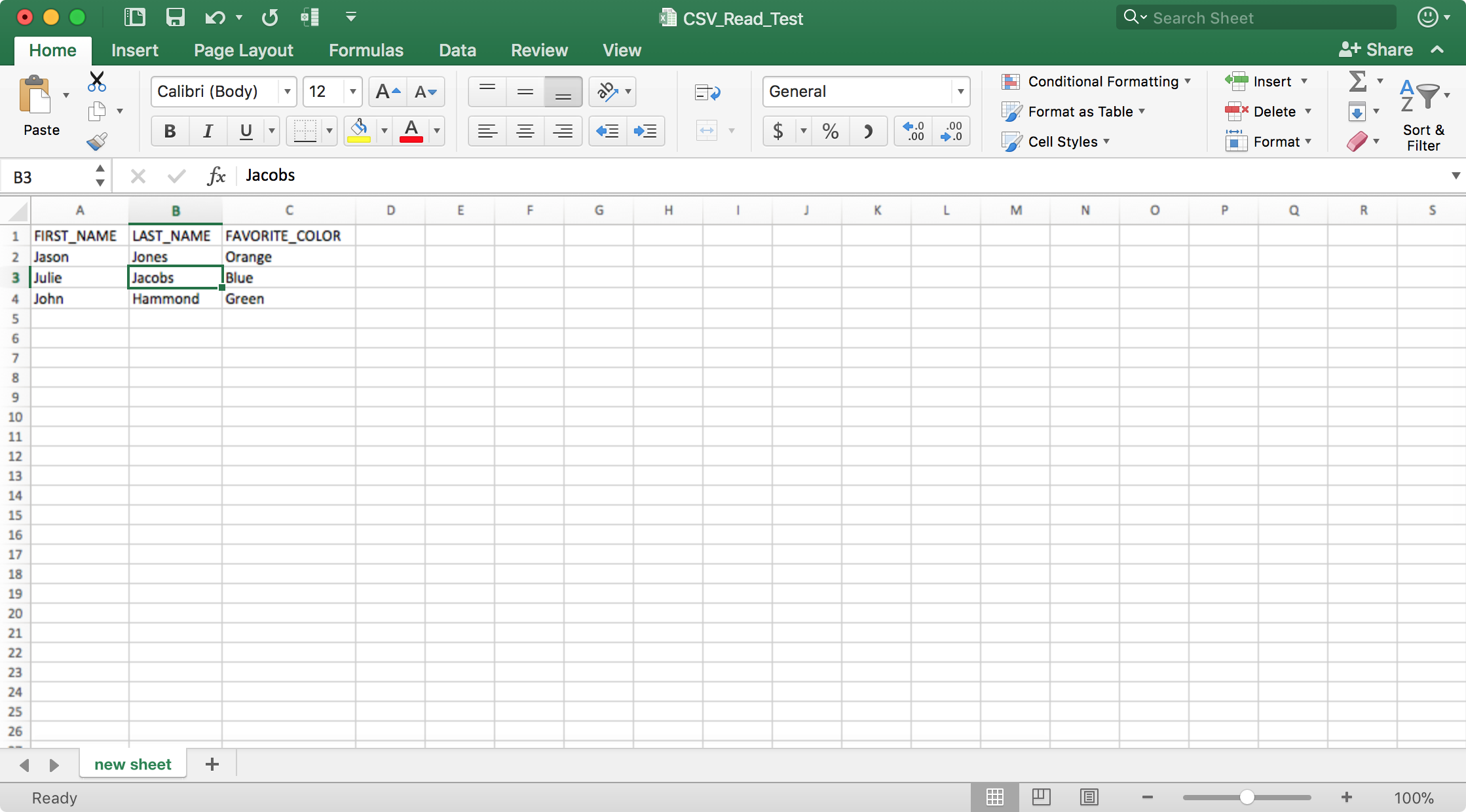
Output when downloading to Excel file

You might think that we are achieving Inception-style levels of recursion by downloading a CSV file by way of JDBC by way of another CSV file, but remember that the output has been filtered according to our query. And further: the data is now available via true drill-through (after deploying the drill-through definitions to Essbase of course)!

Performance Notes

I tested this with a real-world CSV file with over half a million rows. Returning the entire file takes about 15 seconds on my machine. I think this is mostly normal page rendering time as opposed to the CSV reading process taking an inordinate amount of time. When I narrow down the query with three WHERE clauses and have 144 output rows, the drill-through results come back in about a second – so the performance even when scanning a somewhat large CSV file seems quite acceptable and even on-par with a traditional relational database.

Misc

There are some additional options on H2’s CSVREAD functionaliy that can give you more control over how the CSV file is read and parsed, in case you need more flexibility with delimiters, newline characters, and things like that.

Summary

I hope you enjoyed this “off the beaten path” Drillbridge use case. In principle, this should work out of the box with both the free (Community Edition) of Drillbridge as well as the licensed version, Drillbridge Plus. Although the ideal drill-through situation might be one where a true relational database is being queried, I know from experience that there are a non-trivial amount of workaround solutions out there, such as like this one that uses Access, that could be quickly and easily upgraded to something vastly more user-friendly and agile. Please don’t hesitate to reach out if you have any questions.

Speed up ASO SQL data loads by using multiple rules files

Just another quick post today about possibly speeding up data loads to an ASO database when loading from SQL. I got on a quick call with a former colleague that was looking to gain a little more performance on their load process to a massive ASO database, and the first thing that jumped out at me was that I recall you can do parallel loads with some native MaxL syntax.

Here’s a quick example of the syntax:


import database $APPLICATION.$DATABASE data
connect as $SQL_USER identified by $SQL_PW
using multiple rules_file $RULE1, $RULE2, $RULE3, $RULE4, $RULE5
to load_buffer_block starting with buffer_id 100 on error write to "errors.txt";

Basically, you provide multiple rules files (configured for your SQL datasource of course). The rules files are likely to be the same as each other but I suppose it’s possible you might want to partition the data in some logical way to try and speed things up even more.

For example, let’s say that in the code above, we are loading five years of data from a relational database. We might then make it so that each rule is set for this particular year by doing the following things:

  • Set the year in the data header
  • Remove that column from the list of SELECT columns
  • Put a filter/predicate in the WHERE clause on the query
  • Bonus points for using substitution variables in both the header definition and the where clause

Performance in this particular use case went up substantially. It’s my understanding that data loads that were taking an hour are now cut down to 17 minutes. Your mileage may vary, of course.

Let’s Not Forget About Hybrid BSO

That said, I think this can be an effective strategy for trying to squeeze performance out of some ASO cubes that need a smaller load window and you don’t want to go changing a lot of the internals in play. If you’re doing new development, then I strongly, strongly recommend using hybrid BSO (or rather, BSO and making sure the cube is configured properly so as to get the hybrid BSO performance benefits). I have been seeing hybrid BSO cubes absolutely killing it in performance, what with their ability to leverage ASO technology for aggregates, and massive calculation improvements owing to the smaller block sizes and indexes you get from having so many dynamic calc members in dimensions. Plus, you of course get all of the classic/rich/awesome BSO functionality out of the box, like dynamic time series, expense tagging, time balance, and more. These were never very strong areas for ASO and often required a lot of non-optimal workarounds to make users happy.

New webpage for Essbase Java API evolution

A fair bit of my job is dealing with and building solutions around the Essbase Java API. For many years, the Java API has been the premier way to programmatically work with Essbase (compared to say, the C and VB APIs, which have fallen out of favor). As part of this development work, it’s often important to see when (in terms of version) a certain class, method, interface, or other object has been added, modified, removed, or deprecated.

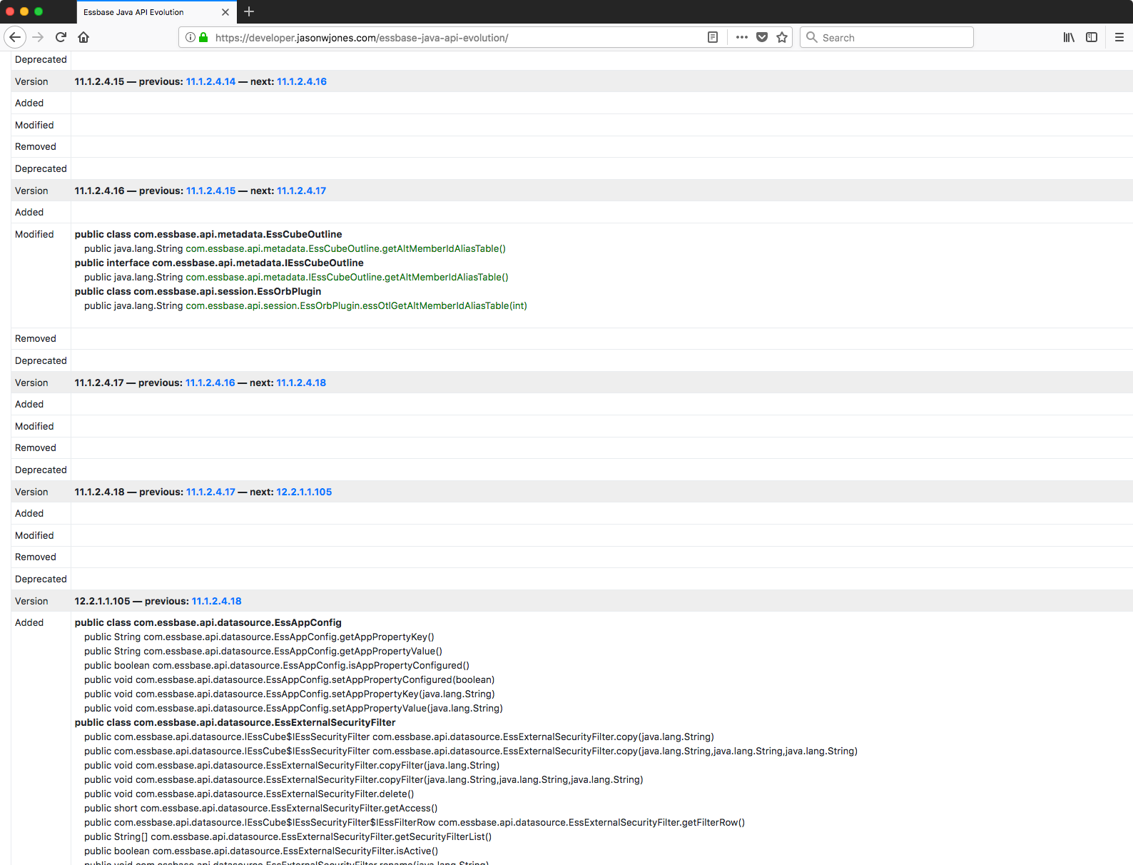
As a bit of a side project, I have been working with a library for comparing Java JARs to each other (japicmp). By processing and interpreting the results of just about every single Essbase Java JAR from 7.0.1, through the 9.x series, multiple 11.x’s, and finally to version 12.2.x, I have come up with something of a master table that shows all of these changes. You can view the initial results of the Essbase JAPI JAR evolution analysis. I’ll probably refresh this and enhance the output as new library versions become available or as I determine that additional insights become useful.

Screenshot from the Essbase Java API evolution analyzer

Besides purely compatibility/feature availability analysis, it’s also interesting to view the changes for other reasons. Often times, features go into the API “under the hood” before they are generally available in the product itself on a more polished basis. This can give insight into features that were being worked on (but were discarded or otherwise changed development plans), and other sort of historical anomalies.

For example, it’s kind of interesting to see the licensing functionality that officially made its debut in the API at version 9.3.0. Some of you long-time and diehard Essbase fans might recall (for better or worse – usually not better) some of the pain around licensing, where the licensing was somewhat a la carte – o be somewhat charitable to Hyperion at the time. This is reflected in the API at the time where you can see that there are many boolean methods that snitch report on licensed counts of CPUs, admin users, users, max connections, named users, Planning users, “restricted” Planning users, and availability of features such as ASO, BSO, app manager, 64-bit, the API, business rules, “crystal”, currency conversion, EDS, EIS, partitions, reports, SQL (for load rules), triggers, and more.

Anyway, if you’re one of the handful of hardcore Essbase Java API developers out there (or otherwise just have weird hobbies), please let me know what you think and if you’d like to see any additions/changes to the output.

Configuring Drillbridge with Financial Reporting Web Studio

Drillbridge works perfectly with Financial Reporting Web Studio – the successor to the desktop-based version of Financial Reporting (also commonly called HFR, FR). FR was stuck with a very archaic client (let’s just say it’s from around the Clinton administration), but it has revamped for the future, with a completely web-based interface now. In retrospect, and based on my interactions with the interface, I think this product overall can be thought of as gap coverage for FR users. It’s not necessarily the place you want to do new development, especially given some of the other shifts/developments in the reporting ecosystem lately. My colleague Opal Alapat has posted some really great thoughts on FR and its place in this ever-changing world, which I encourage you to read.

In the meantime, there are countless current installs of FR that organizations need to support and perhaps transition to this newer incarnation of FR. As with before, Drillbridge works seamlessly to give you and your users advanced drill-through capabilities in Smart View, Hyperion Planning/PBCS, FR, and now FR web. I found that the UI had a few quirks to it, but I’ll walk through a simple example and try to point those out along the way.

First things first, let’s login to Workspace:

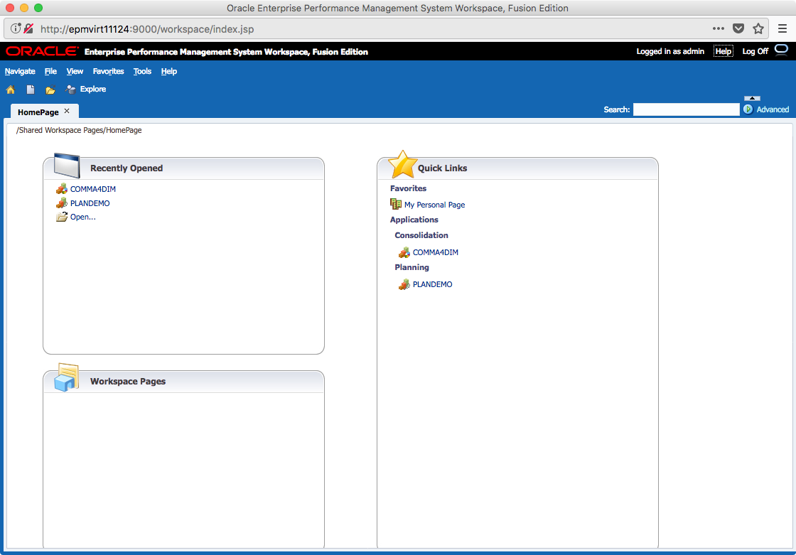
Hyperion Workspace main login page

Default Workspace page

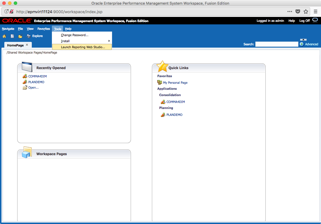
The Tools menu contains our launcher for the web studio:

Hyperion Workspace main screen with Tools menu showing options, including Launch Reporting Web Studio

Launching Reporting Web Studio from Tools menu

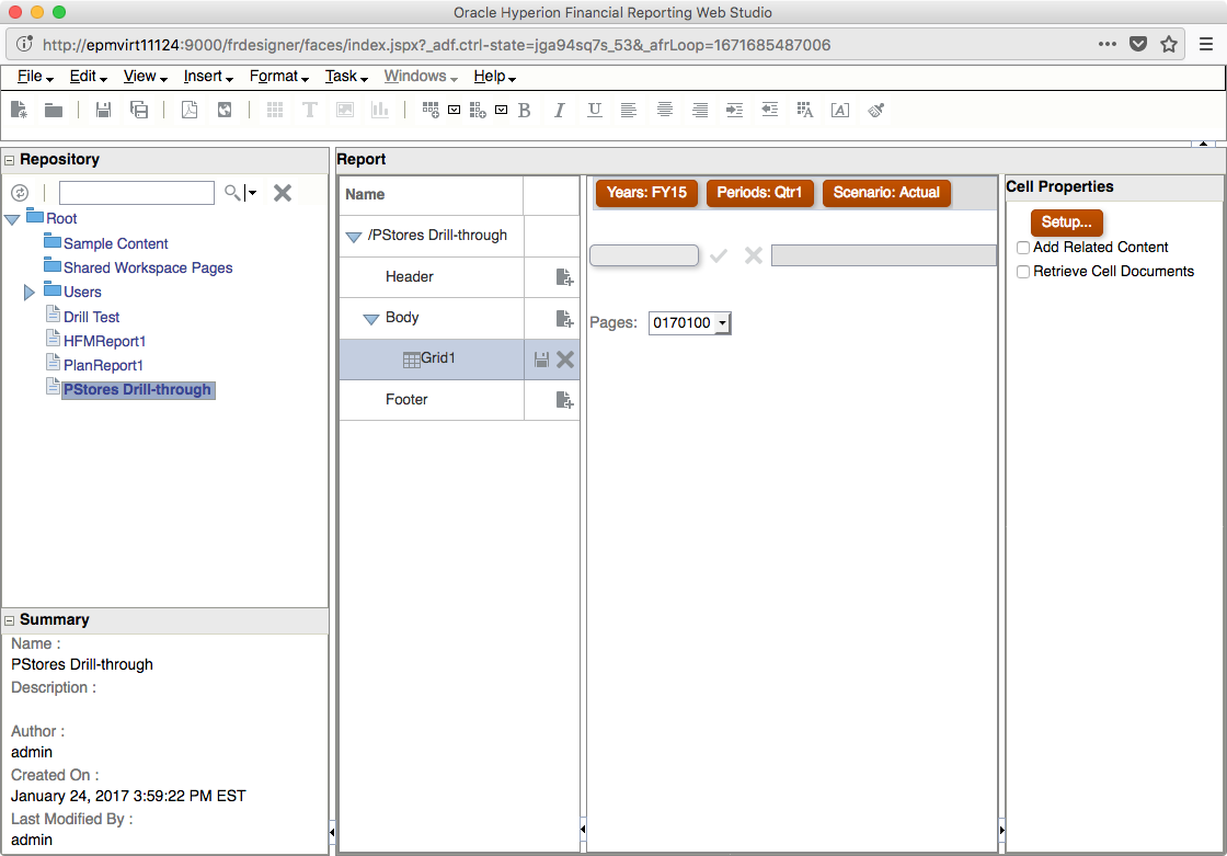
Once we’re there, we should see something like this (results will vary based on your environment of course):

Financial Reporting Web Studio editor page, with a report being edited

FR Web Studio editor editing a particular report, with data cell properties selected

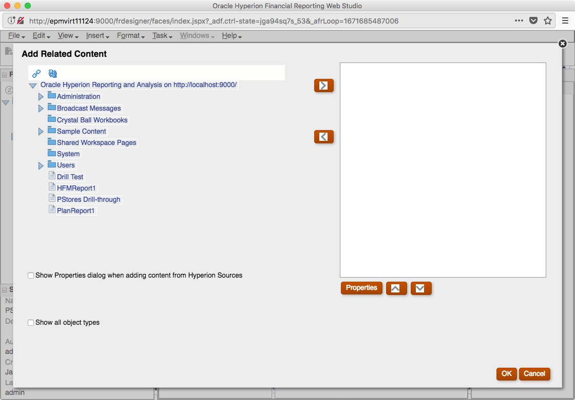
In the preceding screenshot, I have a very simple FR report already opened, and further, it contains a data grid (Grid1). You can’t see it in the above screenshot I have further selected one of the data cells in the Grid1 layout, which has updated the contents of the rightmost pane in the screenshot (Cell Properties). This is where I can setup related content (drill-through). Clicking on the Setup… button brings up the following dialog:

Add Related Content Dialog in Financial Reporting Web Studio

Adding Related Content (notice the chain icon)

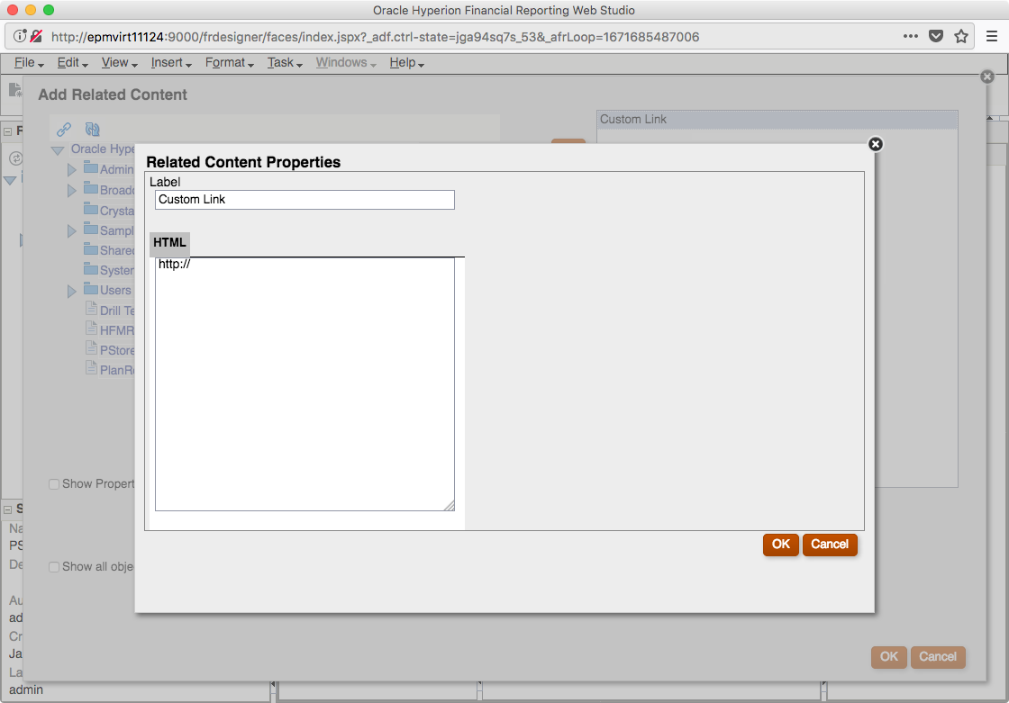
There are no related content definitions, yet, hence the empty list on the right. This is where things got a little funky for me in the UI. It seems that I couldn’t actually edit things in the listbox once I added them, even though it ostensibly let me edit them. I had to remove them and re-add them, and make sure that the title/URL were set exactly right on the first try. Further, the UI is also a little unintuitive in terms of adding custom related content (such as for the Drillbridge definitions), but not too bad. To add a Drillbridge definition, click on the chain/link icon in the top left, then click on the right arrow. This will bring up the following dialog:

Related Content Properties dialog screen on Add Related Content in Financial Reporting Web Studio

Default Related Content properties

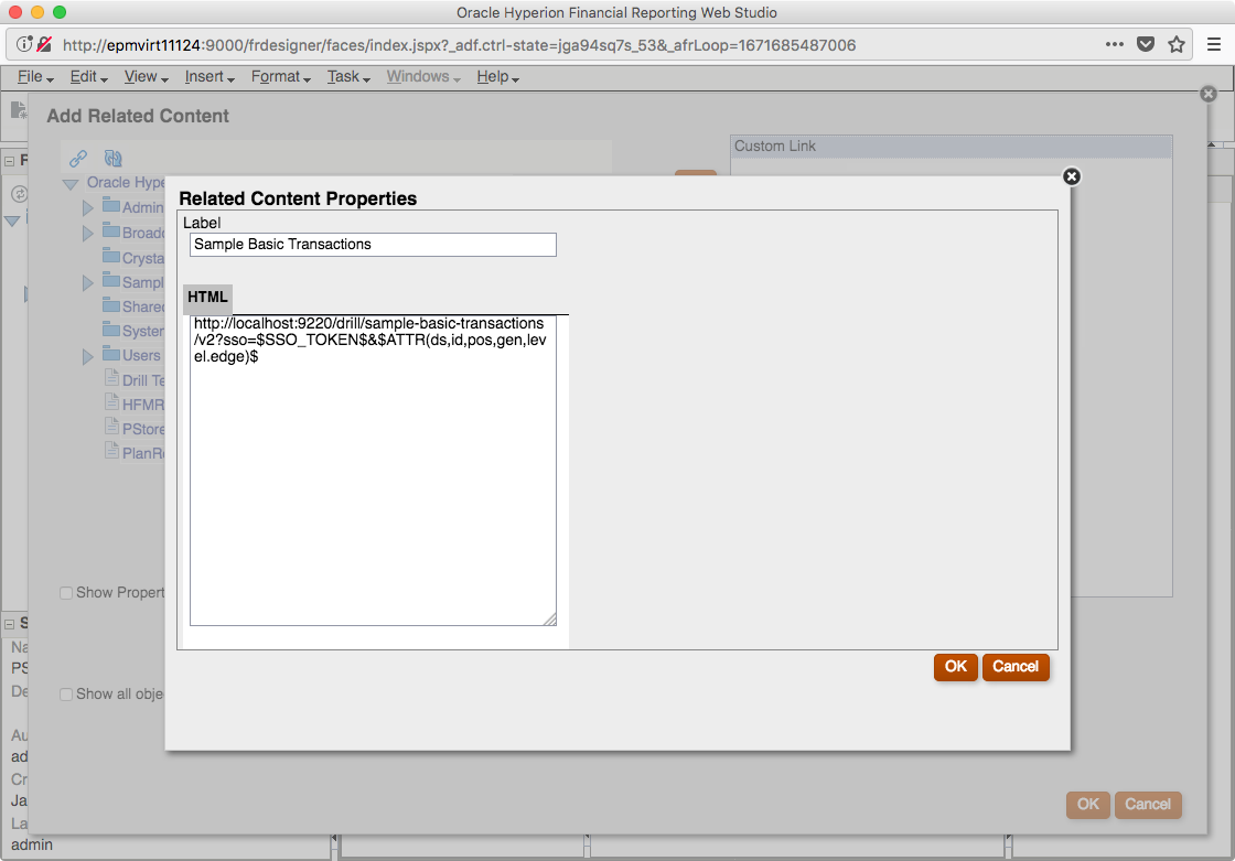
Now we can set the Drillbridge report title (it can be anything you want, it’s just the display value in FR, but you are encouraged to make it the same title as you have set for your Drillbridge definition and deployed to Essbase), and a Drillbridge URL (provided by Drillbridge, or customized by yourself):

Related Content Properties editor filled in with a Drillbridge report title and URL definition

Putting in a Drillbridge title and report URL definition

For reference, here’s that URL:

http://localhost:9220/drill/sample-basic-transactions/v2?sso=$SSO_TOKEN$&$ATTR(ds,id,pos,gen,level.edge)$

Note: don’t use localhost in your environment. I was able to use this because I had a Drillbridge server running on my actual machine (as in my same laptop that was using Firefox to login to FR in the first place) but this should be your actual static Drillbridge server. Also, if you are incredibly eagle-eyed and a Drillbridge aficionado, you might have noticed that rather than specifying a Drillbridge report number in the URL, I’m using the new “logical alias” feature, to specify a more friendly report name of sample-basic-transactions.

This is a really killer feature in Drillbridge that I’ve covered before but I’ll go into briefly. You can give your reports an arbitrary, URL-friendly name (no spaces/special characters) and use that to launch Drillbridge reports now. You can still use the numeric ID if you want, of course. But using the logical alias makes migrations easier, and makes logs a lot easier to read through, among other things. I definitely recommend using this feature if you can.

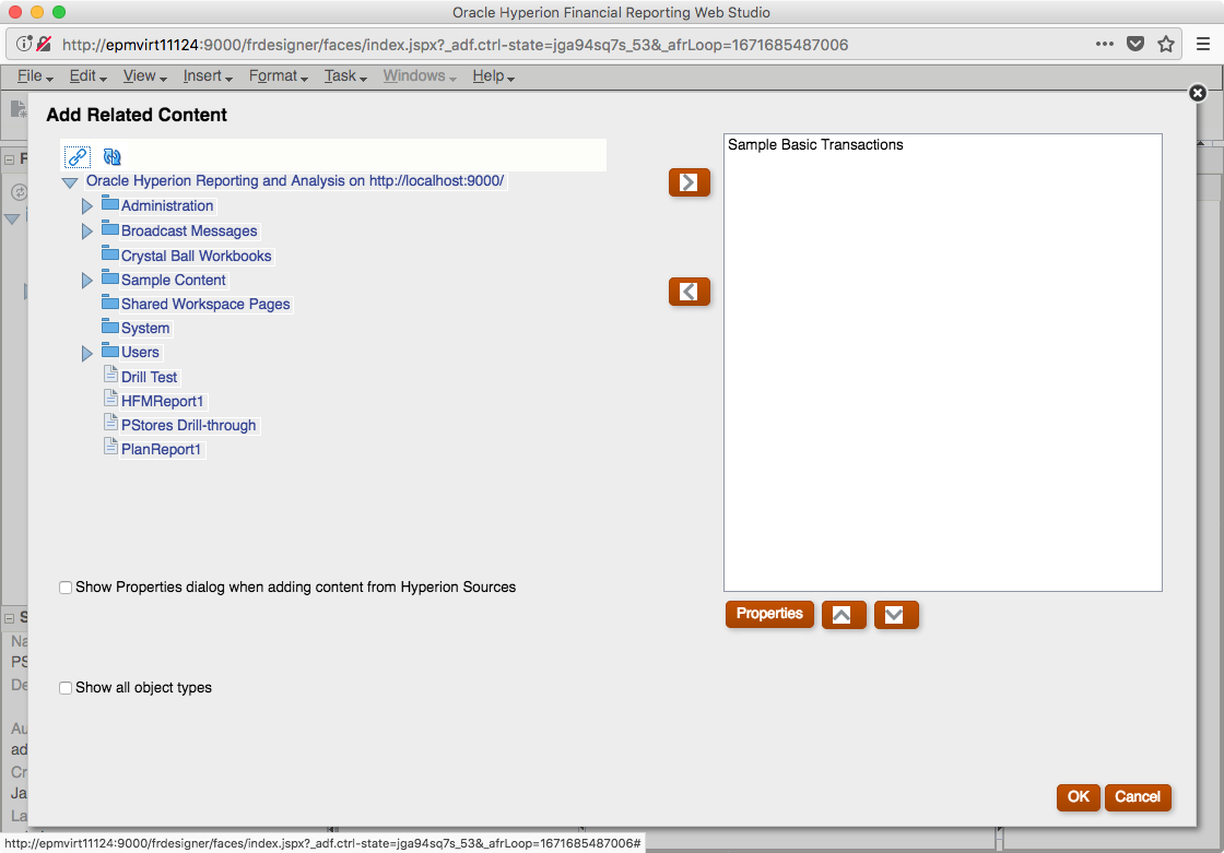
Now we can save the related content by clicking on OK. It’s now added to the list of available related content:

Add Related Content dialog in Financial Reporting Studio with a single drill-through definition

Viewing added Related Content after saving report definition

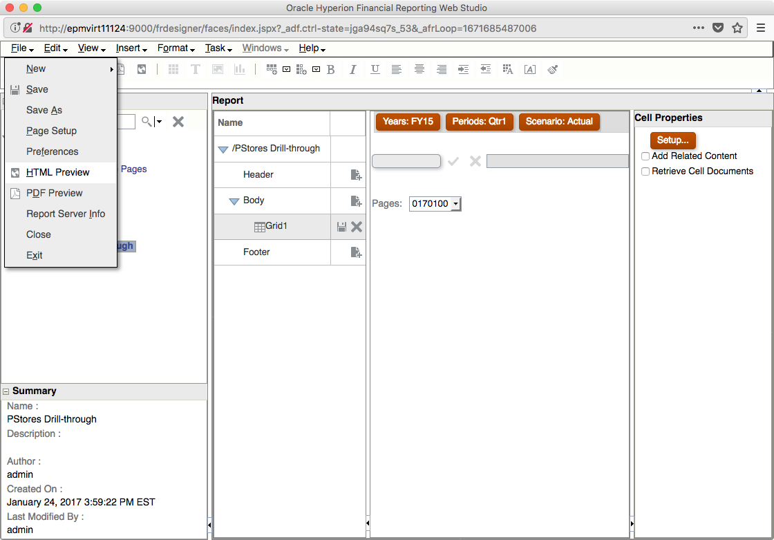
Let’s now go launch an HTML preview of the report by navigating to the File menu and selecting HTML Preview:

Financial Reporting Studio web editor with File menu highlighting the HTML Preview menu option

Launching HTML Preview to test things out

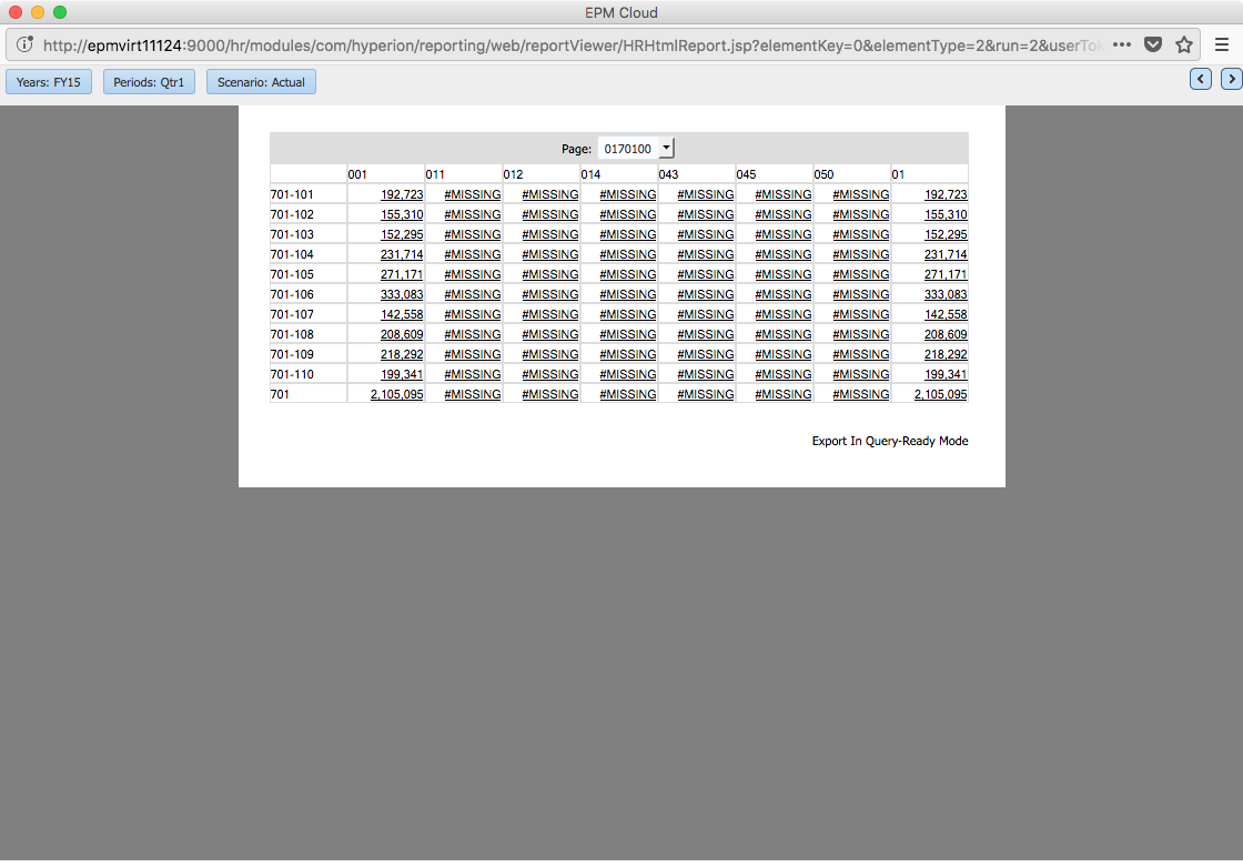
Giving us something like this (notice the hyperlinked data cells):

HTML Preview of a Financial Reporting Web Studio report

HTML preview for a our simple report (notice data cells are hyperlinks)

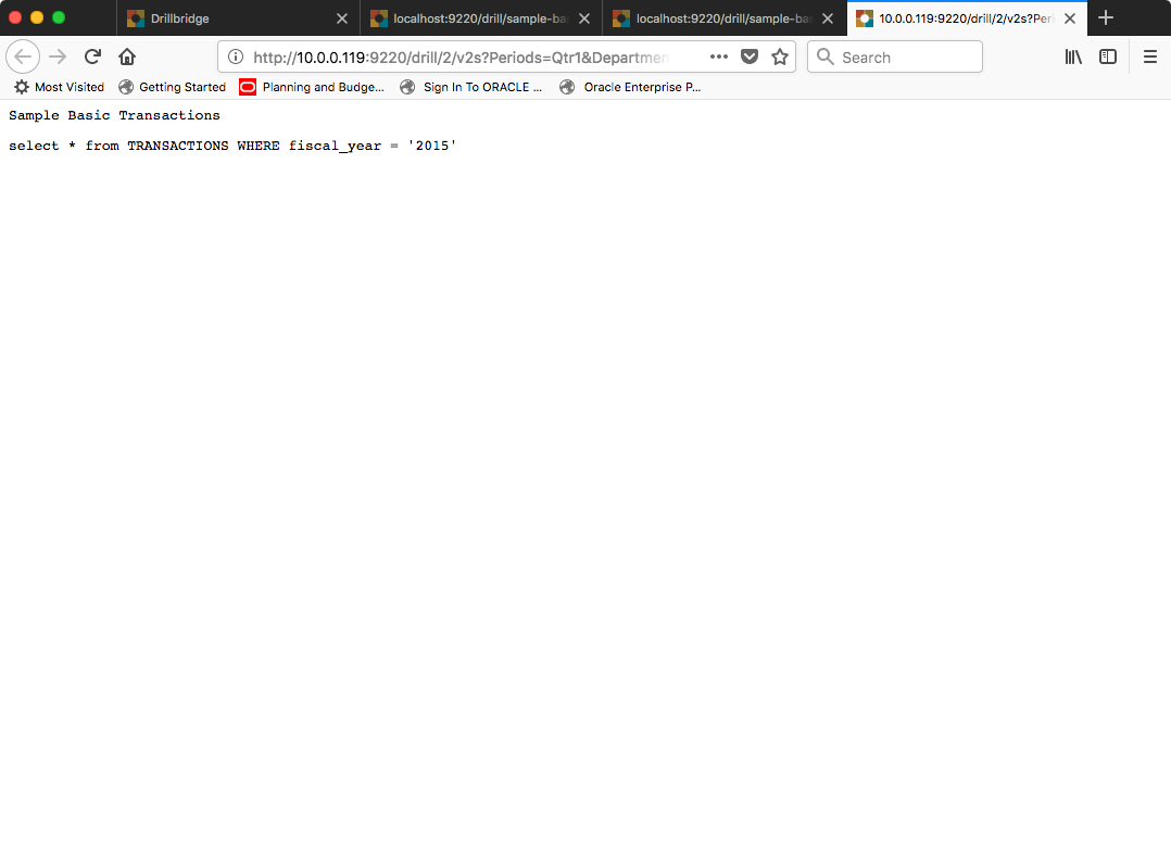
I can now click on one of the data cells to launch the Drillbridge drill-through report. For testing purposes, I have turned the Drillbridge debugging feature (link is primarily about an attribute dimension feature but also contains background on the debug feature) on for this particular report, which means that Drillbridge will just generate the SQL query and render that to the screen, without actually executing the query. This is really useful for testing and development. Let’s see what query Drillbridge generates:

Firefox Web Browser showing a Drillbridge report with debugging turned on

The resulting Drillbridge report (note that debugging is turned on)

This looks good. Notice that the FY15 member was translated to 2015, as per this report’s query definition (to strip the FY prefix and prepend the value of 20). I’ll now turn off debugging for this report and launch it again:

Firefox web browser showing a Drillbridge report that contains no data

Drillbridge report with debugging turned off (intentionally has no data)

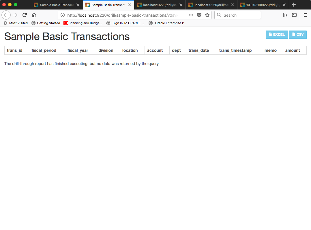
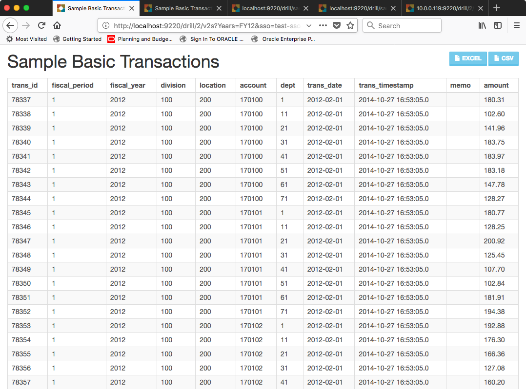
As it turns out, there is no data in my test database for this particular intersection, which is fine. Nicely enough, one of the newer refinements to Drillbridge includes some helpful text such that when the query finishes, if there was no data, Drillbridge will indicate as much. This is a small but helpful usability improvement to prevent use-cases where a user might think a long-running query is executing, but in fact there is no data). Let’s change to a different year member and launch the report one more time:

Firefox web browser showing a typical Drillbridge report named Sample Basic Transactions

Changing to a POV with data and relaunching

Success!

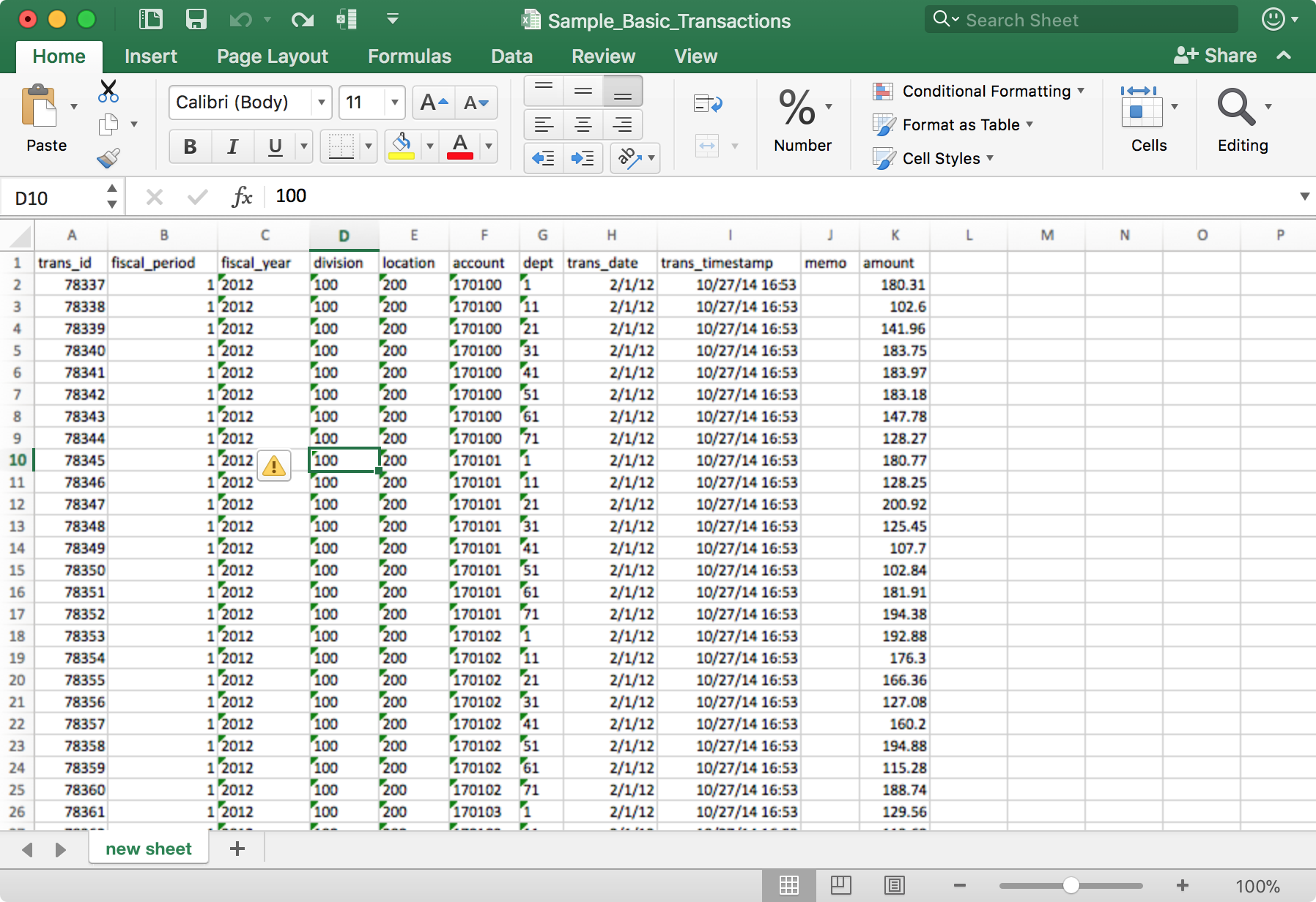
And of course, as always I can download the data to Excel with just a click:

Drillbridge report data downloaded to Excel

Downloading to Excel

Wrapping Up

I hope you found this article on configuring Drillbridge with Financial Reporting’s fully web-capable incarnation to be interesting. Drillbridge continues to be an incredibly useful tool for helping companies quickly enhance the value of their cubes, whether on-premise or on the cloud – please don’t hesitate to reach out to me if you have any questions.